Inverse CDF Sampling

Inverse CDF sampling is a method for obtaining samples from both discrete and continuous probability distributions that requires the CDF to be invertible. The method assumes values of the CDF are Uniform random variables on $[0, 1]$. CDF values are generated and used as input into the inverted CDF to obtain samples with the distribution defined by the CDF.

Discrete Distributions

A discrete probability distribution consisting of a finite set of $N$ probability values is defined by,

$\{p_1,\ p_2,\ \ldots,\ p_N\}\ \ \ \ \ (1),$

with $p_i\ \geq\ 0, \ \forall i$ and $\sum_{i=1}^N{p_i} = 1$. The CDF specifies the probability that $i \leq n$ and is given by,

$P(i\ \leq\ n)=P(n)=\sum_{i=1}^n{p_i},$

For a given CDF value, $U$, The equation for $P(n)$ can always be inverted by evaluating it for each $n$ and searching for the smallest value of $n$ that satisfies, $P(n)\ \geq\ U$. It follows that generated samples determined from $U \sim \textbf{Uniform}(0, 1)$ will have distribution $(1)$ since the intervals $P(n)-P(n-1) = p_n$ are uniformly sampled.

Consider the distribution,

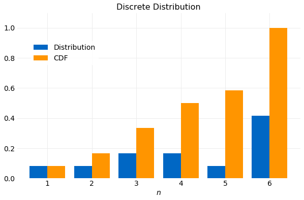
$\left\{\frac{1}{12},\ \frac{1}{12},\ \frac{1}{6},\ \frac{1}{6},\ \frac{1}{12},\ \frac{5}{12} \right\} \ \ \ \ \ (2)$ It is shown in the following plot with its CDF. Note that the CDF is a monotonically increasing function.

A sampler using the Inverse CDF method with target distribution specified in $(2)$ implemented in Python is shown below.

import numpy

n = 10000
df = numpy.array([1/12, 1/12, 1/6, 1/6, 1/12, 5/12])
cdf = numpy.cumsum(df)

samples = [numpy.flatnonzero(cdf >= u)[0] for u in numpy.random.rand(n)]

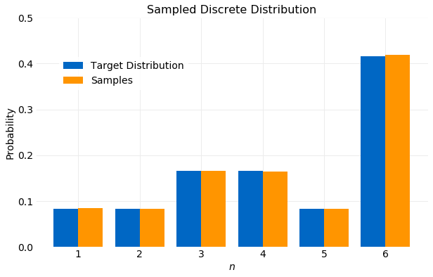
The program first stores the CDF computed from the partial sums $P(n)$ in an array. Next, CDF samples using $U \sim \textbf{Uniform}(0, 1)$ are generated. Finally, for each sampled CDF value, $U$, the array containing $P(n)$ is scanned for the smallest value of $n$ where $P(n)\ \geq\ U$. The resulting values of $n$ will have the target distribution $(2)$. This is shown in the figure below.

A measure of convergence of the samples to the target distribution can be obtained by comparing the cumulative moments of the distribution computed from the samples with the target value of the moment computed analytically. In general for a discrete distribution the first and second moments are given by,

$\begin{aligned} \mu & = \sum_{i=1}^N ip_i\\ \sigma^2 & = \sum_{i=1}^N i^2p_i - \mu^2, \end{aligned}$

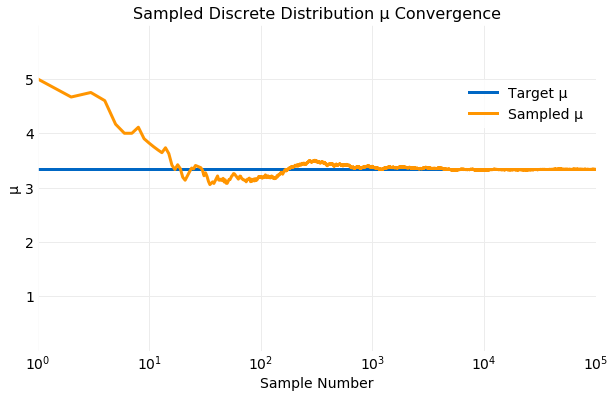
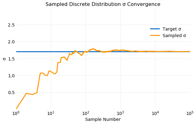
In the following two plots the cumulative values of $\mu$ and $\sigma$ computed from the samples generated are compared with the target values using the equations above. The first shows the convergence of $\mu$ and the second the convergence of $\sigma$. Within only $10^3$ samples both $\mu$ and $\sigma$ computed from samples is comparable to the target value and by $10^4$ the values are indistinguishable.

The number of operations required for generating samples using Inverse CDF sampling from a discrete distribution will scale $O(N_{samples}N)$ where $N_{samples}$ is the desired number of samples and $N$ is the number of terms in the discrete distribution.

It is also possible to directly sample distribution $(2)$ using the multinomial sampler from numpy,

import numpy

n = 10000
df = numpy.array([1/12, 1/12, 1/6, 1/6, 1/12, 5/12])
samples = numpy.random.multinomial(n, df, size=1)/n

Continuous Distributions

A continuous probability distribution is defined by the PDF, $f_X(x)$, where $f_X(x) \geq 0,\ \forall x$ and $\int_{-\infty}^{\infty} f_X(x) dx = 1$. The CDF is a monotonically increasing function that specifies the probability that $X\ \leq\ x$, namely,

$P(X \leq x) = F_X(x) = \int_{-\infty}^{x} f_X(w) dw.$

Theory

To prove that Inverse CDF sampling works for continuous distributions it must be shown that,

$P[F_X^{-1}(U)\ \leq\ x] = F_X(x) \ \ \ \ \ (3),$

where $F_X^{-1}(x)$ is the inverse of $F_X(x)$ and $U \sim \textbf{Uniform}(0, 1)$.

A more general result needed to complete this proof is obtained using a change of variable on a CDF. If $Y=G(X)$ is a monotonically increasing invertible function of $X$ it will be shown that,

$P(X\ \leq\ x) = P(Y\ \leq\ y) = P[G(X)\ \leq\ G(x)]. \ \ \ \ \ (4)$

To prove this note that $G(x)$ is monotonically increasing so the ordering of values is preserved for all $x$,

$X\ \leq\ x\ \implies\ G(X)\ \leq\ G(x).$

Consequently, the order of the integration limits is maintained by the transformation. Further, since $y=G(x)$ is invertible, $x = G^{-1}(y)$ and $dx = (dG^{-1}/dy) dy$, so

$\begin{aligned} P(X\ \leq\ x) & = \int_{-\infty}^{x} f_X(w) dw \\ & = \int_{-\infty}^{y} f_X(G^{-1}(z)) \frac{dG^{-1}}{dz} dz \\ & = \int_{-\infty}^{y} f_Y(z) dz \\ & = P(Y\ \leq\ y) \\ & = P[G(X)\ \leq\ G(x)], \end{aligned}$

where,

$f_Y(y) = f_X(G^{-1}(y)) \frac{dG^{-1}}{dy}$

For completeness consider the case where $Y=G(X)$ is a monotonically decreasing invertible function of $X$ then,

$X\ \leq\ x\ \implies\ G(X)\ \geq\ G(x),$

it follows that,

$\begin{aligned} P(X\ \leq x) & = \int_{-\infty}^{x} f_X(w) dw \\ & = \int_{y}^{\infty} f_X(G^{-1}(z)) \frac{dG^{-1}}{dz} dz \\ & = \int_{y}^{\infty} f_Y(z) dz \\ & = P(Y\ \geq\ y) \\ & = P[G(X)\ \geq\ G(x)] \\ & = 1 - P[G(X)\ \leq\ G(x)] \end{aligned}$

The desired proof of equation $(3)$ follows from equation $(4)$ by noting that $U \sim \textbf{Uniform}(0, 1)$ so $f_U(u) = 1$,

$\begin{aligned} P[F_X^{-1}(U)\ \leq\ x] & = P[F_X(F_X^{-1}(U))\ \leq\ F_X(x)] \\ & = P[U\ \leq\ F_X(x)] \\ & = \int_{0}^{F_X(x)} f_U(w) dw \\ & = \int_{0}^{F_X(x)} dw \\ & = F_X(x). \end{aligned}$

Example

Consider the Weibull Distribution. The PDF is given by,

$f_X(x; k, \lambda) = \begin{cases} \frac{k}{\lambda}\left(\frac{x}{\lambda} \right)^{k-1} e^{-\left(x/\lambda\right)^k} & x\ \geq\ 0 \\ 0 & x < 0 \end{cases} \ \ \ \ \ (5)$

where $k\ >\ 0$ is the shape parameter and $\lambda\ >\ 0$ the scale parameter. The CDF is given by,

$F_X(x; k, \lambda) = \begin{cases} 1-e^{\left(\frac{-x}{\lambda}\right)^k} & x\ \geq\ 0 \\ 0 & x\ <\ 0. \end{cases}$

The CDF can be inverted to yield,

$F_X^{-1}(u; k, \lambda) = \begin{cases} \lambda\ln\left(\frac{1}{1-u}\right)^{\frac{1}{k}} & 0\ \leq\ u\ \leq 1 \\ 0 & u\ <\ 0 \text{ or } u\ >\ 1. \end{cases}$

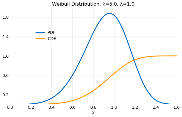
In the example described here it will be assumed that $k=5.0$ and $\lambda=1.0$. The following plot shows the PDF and CDF using these values.

The sampler implementation for the continuous case is simpler than for the discrete case. Just as in the discrete case CDF samples with distribution $U \sim \textbf{Uniform}(0, 1)$ are generated. The desired samples with the target $\textbf{Weibull}$ distribution are then computed using the CDF inverse. Below an implementation of this procedure in Python is given.

import numpy

k = 5.0
λ = 1.0
nsamples = 100000

cdf_inv = lambda u: λ * (numpy.log(1.0/(1.0 - u)))**(1.0/k)
samples = [cdf_inv(u) for u in numpy.random.rand(nsamples)]

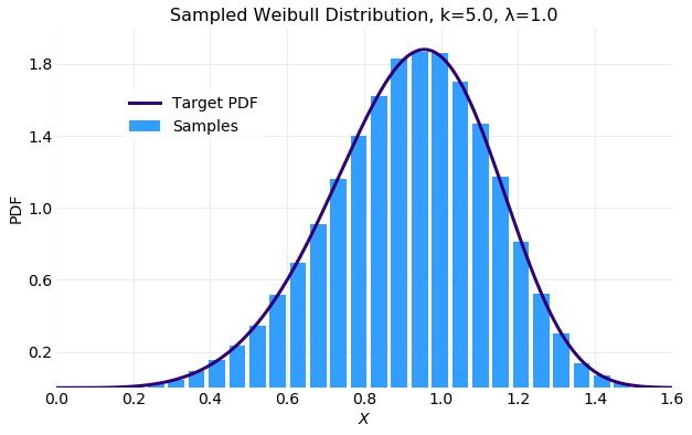
The following plot compares a histogram of the samples generated by the sampler above and the target distribution (5). The fit is quite good. The subtle asymmetry of the $\textbf{Weibull}$ distribution is captured.

The first and second moments for the $\textbf{Weibull}$ distribution are given by,

$\begin{aligned} \mu & = \lambda\Gamma\left(1+\frac{1}{k}\right) \\ \sigma^2 & = \lambda^2\left[\Gamma\left(1+\frac{2}{k}\right)-\left(\Gamma\left(1+\frac{1}{k}\right)\right)^2\right], \end{aligned}$

where $\Gamma(x)$ is the Gamma function.

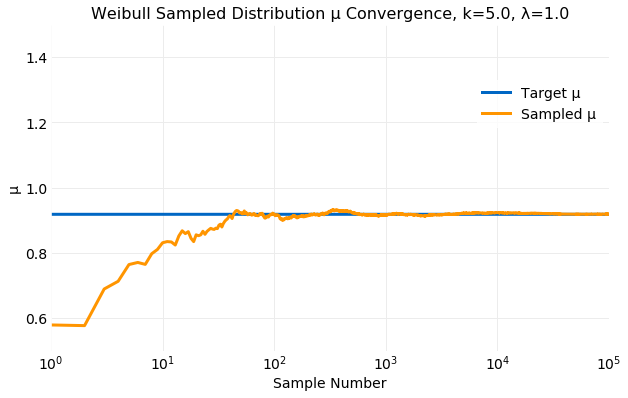
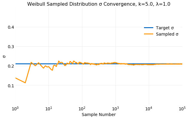
The following two plots compare the cumulative values of $\mu$ and $\sigma$ computed from sampling of the target distribution $(5)$ with the values from the equations above. The first shows the convergence of $\mu$ and the second the convergence of $\sigma$. Within only $10^3$ samples both $\mu$ and $\sigma$ computed from samples are comparable to the target values and by $10^4$ the values are indistinguishable.

Performance

Any continuous distribution can be sampled by assuming that $f_X(x)$ can be approximated by the discrete distribution, $\left\{f_X(x_i)\Delta x_i \right\}_N$ for $i=1,2,3,\ldots,N$, where $\Delta x_i=(x_{max}-x_{min})/(N-1)$ and $x_i = x_{min}+(i-1)\Delta x_i$. This method has disadvantages compared to using Inverse CDF sampling on the continuous distribution. First, a bounded range for the samples must be assumed when in general the range of the samples can be unbounded while the Inverse CDF method can sample an unbounded range. Second, the number of operations required for sampling a discrete distribution scales $O(N_{samples}N)$ but sampling the continuous distribution is $O(N_{samples})$.

Conclusions

Inverse CDF Sampling provides a method for obtaining samples from a known target distribution using a sampler with a $\textbf{Uniform}(0, 1)$ distribution that requires the target distribution be invertible. Algorithms for both the discrete and continuous cases were analytically proven to produce samples with distributions defined by the CDF. Example implementations of the algorithms for both distribution cases were developed. Samples produced by the algorithms for example target distributions were favorably compared. Mean and standard deviations computed from generated samples converged to the target distribution values in $O(10^3)$ samples. The continuous sampling algorithm was shown to be more performant than the discrete version. The discrete version required $O(N_{samples}N)$ operations while the continuous version required $O(N_{samples})$ operations.