Bivariate Normal Distribution
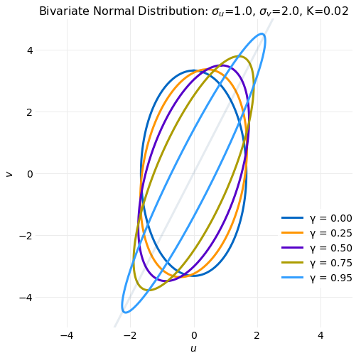
The Bivariate Normal Distribution is an often used multivariable distribution because it provides a simple model of correlated random variables. Here it is derived by application of a linear transformation and a multivariate change of variables to the distribution of two independent unit normal, , random variables. To provide background a general expression for change of variables of a bivariate integral is discussed and then used to obtain the Bivariate Normal Distribution. The Marginal and Conditional distributions are next computed and used to evaluate the first and seconds moments, correlation coefficient and conditional expectation and conditional variance. Finally, the variation in the shape of the distribution and transformation as the distribution parameters are varied is discus... read more
Metropolis Hastings Sampling
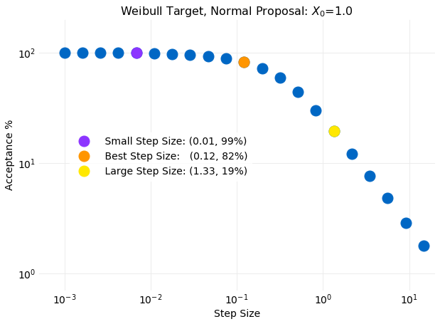
Metropolis Hastings Sampling is a method for obtaining samples for a known target probability distribution using samples from some other proposal distribution. It is similar to Rejection Sampling in providing a criteria for acceptance of a proposal sample as a target sample but instead of discarding the samples that do not meet the acceptance criteria the sample from the previous time step is replicated. Another difference is that Metropolis Hastings samples are modeled as a Markov Chain where the target distribution is the Markov Chain Equilibrium Distribution. As a consequence the previous sample is used as part of the acceptance criteria when generating the next sample. It will be seen this has the advantage of permitting adjustment of some proposal distribution parameters as each sample is generated, which in effect eliminates parameter inputs.
This is is an improvement over Rejection Sampling, where it was previously shown that slight variations in proposal distribution parameters can significantly impact performance. A downside of the Markov Chain representation is that autocorrelation can develop in the samples which is not the case in Rejection Sampl... read moreDiscrete Cross Correlation Theorem
The Cross Correlation Theorem is similar to the more widely known Convolution Theorem. The cross correlation of two discrete finite time series and is defined by,
where is called the time lag. Cross correlation provides a measure of the similitude of two time series when shifted by the time lag. A direct calculation of the cross correlation using the equation above requires operations. The Cross Correlation Theorem provides a method for calculating cross correlation in operations by use of the Fast Fourier Transform. Here the theoretical background required to understand cross correlation calculations using the Cross Correlation Theorem is discussed. Example calculations are performed and different implementations using the FFT libraries in
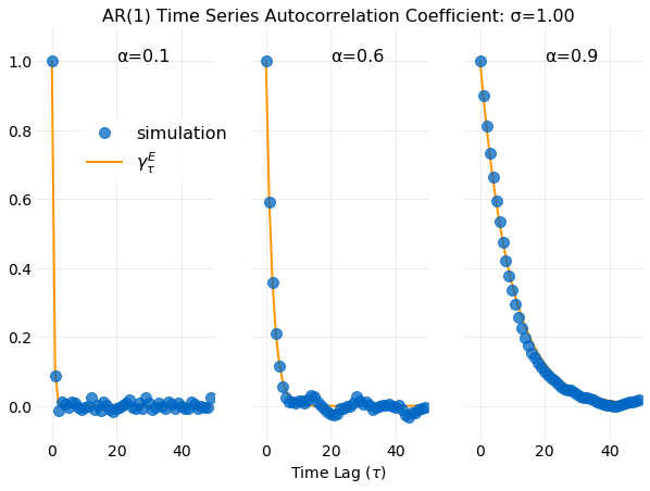
numpycompared. The important special case of the cross correlation called Autocorrelation is addressed in ... read moreContinuous State Markov Chain Equilibrium
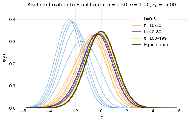
A Markov Chain is a sequence of states where transitions between states occur ordered in time with the probability of transition depending only on the previous state. Here the states will be assumed a continuous unbounded set and time a discrete unbounded set. If the set of states is given by, , the probability that the process will be in state at time , denoted by , is referred to as the distribution. Markov Chain equilibrium is defined by , that is, as time advances becomes independent of time. Here a solution for this limit is discussed and illustrated with examp... read more
Discrete State Markov Chain Equilibrium
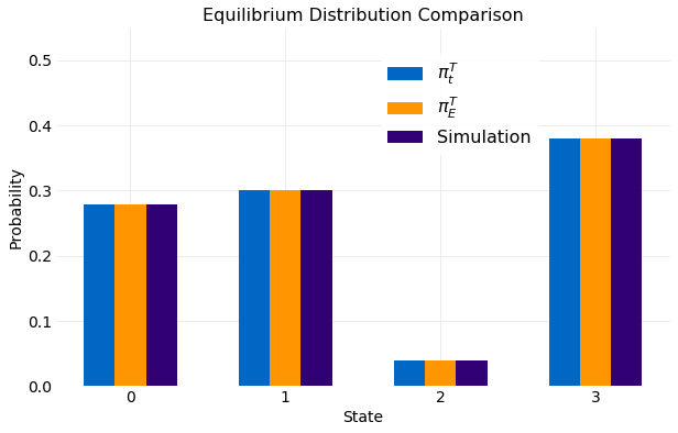
A Markov Chain is a sequence of states where transitions between states occur ordered in time with the probability of transition depending only on the previous state. Here the states will be assumed a discrete finite set and time a discrete unbounded set. If the set of states is given by the probability that the process will be in state at time is denoted by , referred to as the distribution. Markov Chain equilibrium is defined by , that is, as time advances
becomes independent of time. Here a solution for this limit is discussed and illustrated with examp... read more