The Bivariate Normal Distribution is an
often used multivariable distribution because it provides a simple model of correlated
random variables. Here it is derived by application of a linear transformation
and a multivariate change of variables to the distribution of two independent unit normal,
Normal(0,1), random variables. To provide background a general
expression for change of variables of a bivariate integral is discussed and then used to
obtain the Bivariate Normal Distribution. The Marginal and Conditional distributions are next
computed and used to evaluate the first and seconds moments, correlation coefficient
and conditional expectation and conditional variance.
Finally, the variation in the shape of the distribution and transformation as the distribution parameters
are varied is discussed.
Bivariate Change of Variables
Consider the PDF of a single variable, f(x), and the transformation,
x=x(y) which is assumed monotonically increasing.
The PDF of the transformed variable is given by,
g(y)=f(x(y))dydx.
This result follows by performing a change of variables to the CDF,
P(X≤x)=∫−∞xf(w)dw=∫−∞yf(x(w))dwdxdw=P(Y≤y)
where use was made of,
dx=dydxdy.
The dx/dy term scales dy appropriately
to conserve the differential length. In two dimensions a similar but more complicated thing happens.
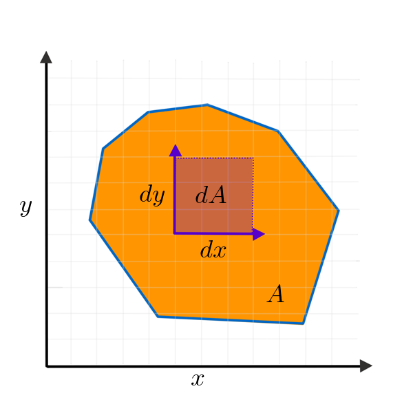
Consider the bivariate PDF, f(x,y), with CDF,
P({X,Y}∈A)=∫Af(x,y)dA,(1)
which defines an integration over a region computing the probability that X and
Y are both in the region A. The figure below provides an illustration for a Cartesian Coordinate System
where dA=dxdy.
To go further a geometric result relating the Cross Product of two vectors to the area of the
parallelogram enclosed by the vectors is needed. This topic is discussed in the following section.
Cross Product as Area
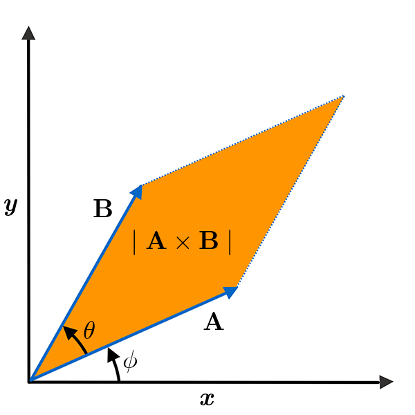
Consider two vectors A and B
separated by an angle θ and rotated by and angle
ϕ as shown in the following figure.
The vector components projected along the x and
y unit vectors is given by,
The cross product of two vectors is another vector perpendicular to both vectors. For the figure
above, that direction is perpendicular to the plane of the page, call it z.
The cross product is then defined by the determinate
computed from the components of the two vectors and projected along
z,
which is the area of the parallelogram indicated by orange in the figure above.
sinθ can be assumed positive since
θ can always be chosen such that
0≤θ≤π.
Bivariate Jacobian
Consider the following coordinate transformation between two coordinate systems defined by the
variables (x,y) and (u,v),
xy=x(u,v)=y(u,v).(4)
applied to the integral,
∫Af(x,y)dxdy,
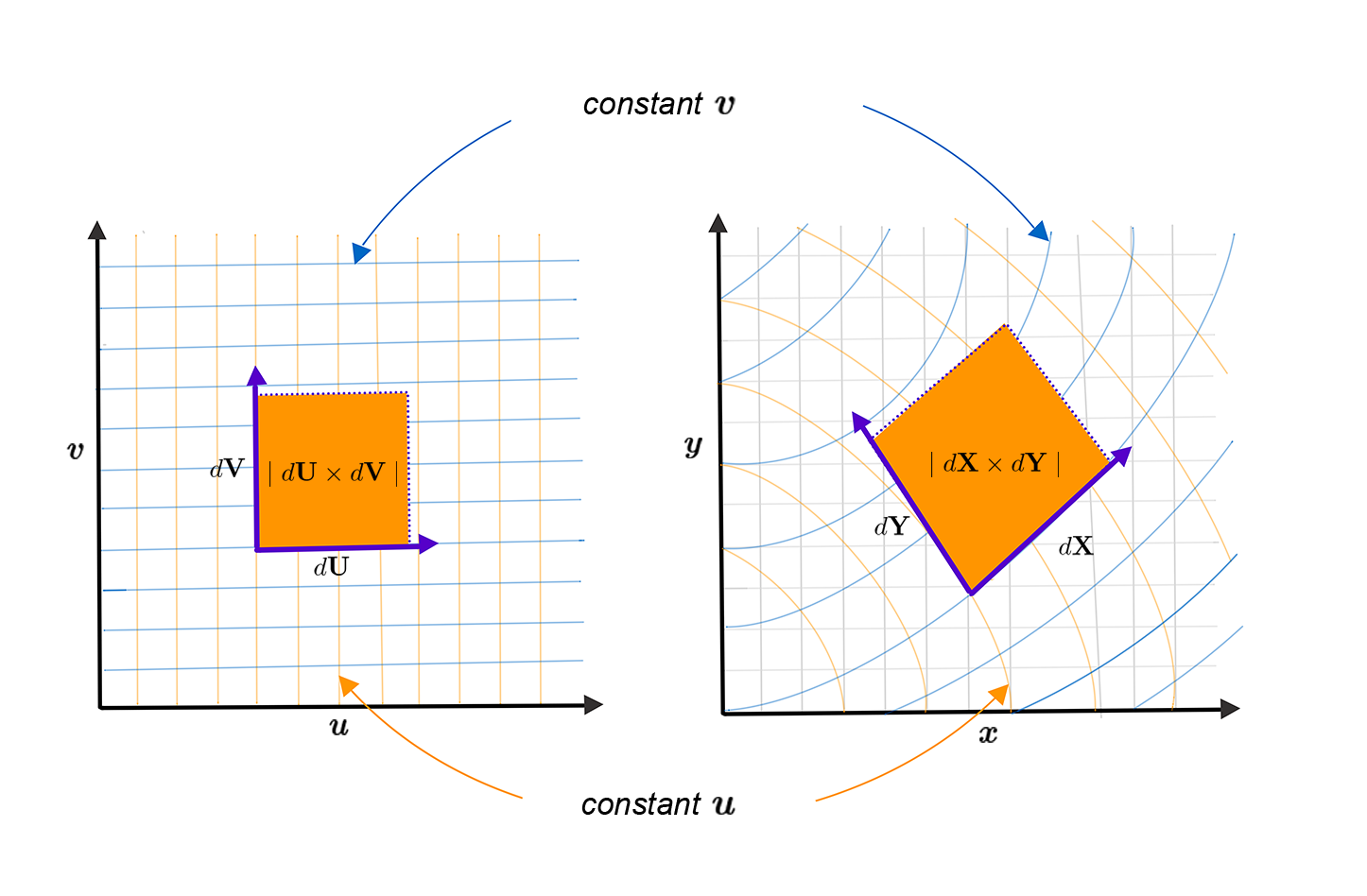
where A is an arbitrary area in (x,y) coordinates. The following figure shows how area elements transform between
(u,v) coordinates
and (x,y) coordinates when equation
(4) is applied. The left side of the figure shows the
(u,v)Cartesian Coordinate System.
In this system vertical lines of constant u
are colored orange and horizontal lines of constant v blue. The right side
of the figure illustrates how equation (4) maps lines of constant
u and v onto
(x,y) coordinates. The lines of constant
u and v
can be curved and not aligned with the (x,y)
Cartesian coordinates as shown in the figure. The transformed
(u,v) coordinates in this case are Curvilinear.
Consider the differential area elements indicated by orange in the figure. In the
(u,v)
Cartesian coordinates the differential area element is given by dA=dudv but
in (x,y) coordinates differentials defining the area are not orthogonal so the element is distorted. In the infinitesimal limit it
will become a parallelogram with area given by the cross product of dX
and dY which are tangent vectors to the curves of constant
v and u respectively at the origin
point of the vectors. To compute the cross product expressions for the differentials are required.
The components of the differentials are computed from transformation
(4) by assuming v is constant for
dX and u is constant for
dY. It follows that,
dXdY=∂u∂xdux+∂u∂yduy=∂v∂xdvx+∂v∂ydvy.
The cross product of the differentials above is given by,
In general the determinate of a matrix equals the determinate of the transpose of the matrix. It follows
that the area element in (u,v)
coordinates is given by,
dA=∣dX×dY∣=∣J∣dudv.
∣J∣ will scale the differential area dudv
by the amount required by the transform to conserve the area in a manner similar to that seen for a
single variable length is conserved.
Finally the transform of the bivariate integral in equation (1) is given by,
∫Af(x,y)dxdy=∫A′f(x(u,v),y(u,v))∣J∣dudv,
where A′ is the region obtained by applying (4)
to A.
Bivariate Normal Distribution
The Bivariate Normal Distribution with random variables U and
V is obtained by applying the following linear transformation to
two independent Normal(0,1) random variables
X and Y,
(U−μuV−μv)=(σuσvγ0σv1−γ2)(XY),(5)
where μu, μv,
σu, σv and
γ are scalar constants named in anticipation of
being the mean, standard deviation and correlation coefficient
of the distribution.
An equation for X and Y in terms
U
and V is obtained by inverting the transformation matrix,
With the goal of keeping things simple in the evaluation of equation (8)
the exponential argument term of equation (7),
x2+y2, will first be considered. Use of
the expressions for x(u,v) and y(u,v) from
equation (9) gives,
The first step expands the right most squared term and the last two steps aggregate
(u−μu) and (v−μv)
terms. The Bivariate Normal PDF follows by inserting equations (10)
and (11) into equation (8),
Extension of transform (5) to more than two dimensions is not clear. The
following section will describe a form of the transformation that makes this more apparent.
Matrix Form of Bivariate Normal Distribution
A matrix form for the Bivariate Normal Distribution PDF can be constructed that scales
to higher dimensions. Here the version for two variables is compared with the results of the
previous section and followed by a discussion of extension to an arbitrary number of dimensions.
To begin consider the column vectors,
Y is the column vector of Bivariate Normal Random variables,
μ the column vector of mean values and P is called the
Covariance Matrix. To continue the inverse of the
covariance matrix and its determinate are required. The inverse is given by,
P−1=σ12σ22(1−γ2)1(σ22−γσ1σ2−γσ1σ2σ12),
and the determinate is,
∣P∣=σ12σ22(1−γ2).
Next, consider the product, where (Y−μ)T is the
transpose of (Y−μ),
To determine the linear transformation, analogous to equation (9),
Pij is factored using
Cholesky Decomposition.
In a following section it will be shown that for two variables,
Cov(Yi,Yj)={γσiσjσi2i≠ji=j.
which is equivalent to equation (13).
Bivariate Normal Distribution Properties
The previous sections discussed the derivation of the Bivariate Normal random variables as
linear combinations of independent unit normal
random variables. Linear combinations were constructed by application of a linear transformation
that includes five independent parameters. In this section interpretations of the parameters are
provided and variation in the distribution as the parameters are varied is described. First, the
Marginal Distributions are calculated and it is
shown that four of the distribution parameters correspond to marginal distribution means and standard deviations. Next, the Correlation Coefficient
of the distribution is computed and shown to correspond to the remaining parameter.
In remaining sections how changes in the parameters
affect the distribution shape are considered. This includes an analysis of PDF contours and the linear
transformation used to construct the distribution.
Marginal Distributions
The Marginal Distributions for u and v
are defined by,
g(u)g(v)=∫−∞∞g(u,v)dv=∫−∞∞g(u,v)du,
where g(u,v) is defined by equation (12). First,
consider evaluation of the integral for g(u),
In the first step the u dependence is factored out for
evaluation of the integral over v. The next step completes the
square of the exponential followed by also factoring the introduced u
term from the v integral. This is followed by simplification of the
u exponential argument. Finally, the integral over
v is evaluated yielding a
Normal(μu,σu) distribution. Similarly,
the marginal distribution g(v) is given by,
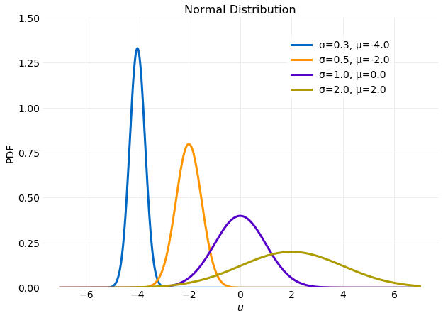
g(v)=∫−∞∞g(u,v)du=2πσv21e−2σv2(v−μv)2,(14)
which is a Normal(μv,σv) distribution. The
plot below shows examples of Normal(μ,σ) as
μ and σ are varied. The effect of
μ is to translate the distribution along the u
axis and σ scales the distribution width.
The mean and variance are now readily determined for both u and
v,
The Conditional Distribution
of a random variable is the distribution obtained by assuming the values of one or more
correlated random variables are known. If the variables are uncorrelated, independent,
the conditional distribution is equivalent to the marginal distribution.
The conditional distribution is useful in the of the calculation of Correlation Coefficient
performed in the following section and in simulation methods such as
Gibbs Sampling.
For the bivariate case the conditional distributions are defined by,
g(u∣v)g(v∣u)=g(v)g(u,v)=g(u)g(u,v)
Using equations (12) and (14),g(u∣v) is evaluated as follows,
In the first step the (v−μv)2 terms are collected and
then the square is completed for the remaining terms. Once again the
(v−μv)2 terms are collected and the finial result obtained,
a Normal distribution.
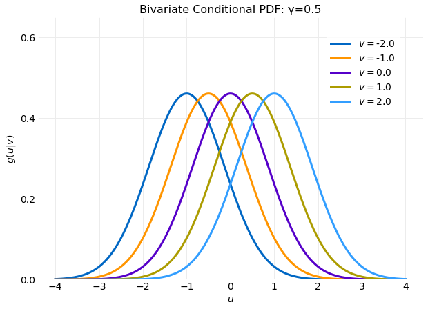
For both u and v the conditional expectation
is a linear function of the conditioned variable. This is illustrated in the following plot
where g(u∣v) is plotted for several values of v.
It is seen that v translates the distribution along the
u axis.
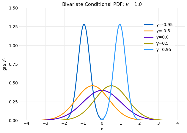
Consider the variation of E[U∣V], E[V∣U],
Var[U∣V] and Var[U∣V] with
γ. For γ=0 each reduces to the
values corresponding to its marginal distribution discussed in the previous section. For both conditional distributions increasing γ leads to decreasing variance resulting in a
sharper peak for the distribution. Additionally, changing the sign of γ causes reflection of the
distribution about the mean. Each of these properties is illustrated on the
plot below where g(u∣v) is plotted for values of
γ ranging from −1 to
1.
Correlation Coefficient
The Cross Correlation of the two random variables
U and V is defined by,
In previous sections it was shown that the free parameters used in the definition of
the Bivariate Normal distribution, equation (12), are its the mean,
variance and correlation coefficient. Here a sketch of the change in shape of the
distribution as these parameters are varied is discussed by evaluating
limits of the parameters for the equation defining the PDF contours.
The following section will describe the convergence to the limits using a numerical analysis.
The equation satisfied by the contours is obtained by setting the argument of the
exponential in equation (12) to a constant, C2,
whereC2 is related to the value of the contour. To develop an
expectation of the behavior the following limits of this equation are considered,
γ→0, γ→±1,
σv/σu→1,
σv/σu→0 and
σv/σu→∞. The variation with
μu and μv produces a translation
which is not as interesting.
First, consider the limit γ→0 which is easily evaluated
using the equation above,
C2=σu2(u−μu)2+σv2(v−μv)2.
This is the equation of an ellipse with axes of length 2Cσu and
2Cσv. The aspect ratio of the ellipse is given by
σv/σu. It follows that in the limit
σv/σu→1 the contour approaches a circle with radius
C and in the limits
σv/σu→0 or
σv/σu→∞ the contour approaches a line along the
u or v axes respectively.
To evaluate the limit γ→±1 it must be noted that
γ2≠1 was assumed in the derivation of inverse of the
Bivariate Transformation, equation (6).
To evaluate the limit it should be evaluated before inverting the transformation defining the distribution,
equation (5). Taking the limit results in a transformation that is valid for
γ2=1,
(U−μuV−μv)=(σu±σv00)(XY).
Evaluation of the equation above gives,
(V−μv)=±σuσv(U−μu).
It follows that as the limit is approached contours will approach a line with slope
±σv/σu. The slope is positive
for positive correlation and negative for negative correlation. In the limit
σv/σu→1 the contour slope
approaches a line with slope ±1 and in the limit
σv/σu→0 or
σv/σu→∞ the contour approaches a line along the
u or v axes respectively which is the same
as obtained in the limit γ→0.
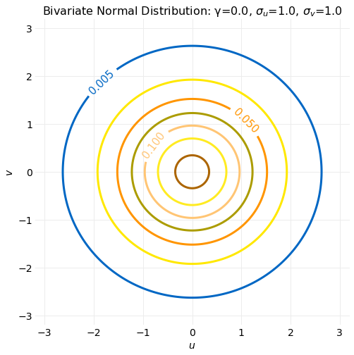
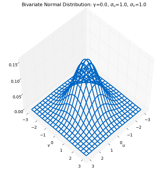
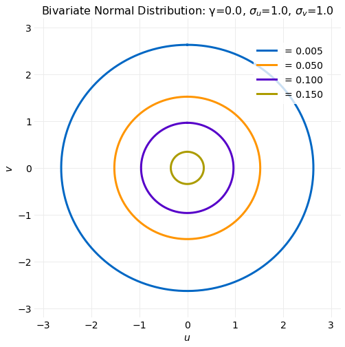
The following two plots show the surface an contour plots for a distribution with
σv/σu=1 and γ=0,
which is the case where u and v are
uncorrelated with equal variances. The contours are circles are previously described.
The surface plot is included to show how poor it is at giving a sense of the distribution shape
though it does assist in imagining the how the contour plot would be projected into the
third dimension.
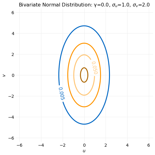
The next plot also has γ=0 but
σv/σu=2. The contours become ellipses with the axis
aligned with the v axis.
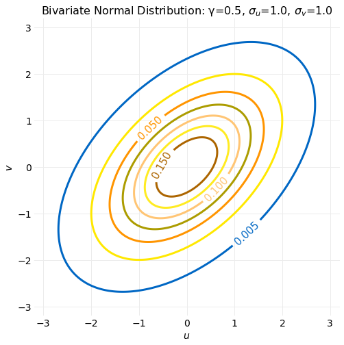
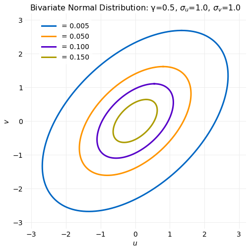
The final plot has γ=0.5 and σv/σu=1.
The contours are symmetric about the line v=u as expected for the limit
γ→±1. If the correlation were negative the contours would be reflected about the v axis and symmetric about the line v=−u.
Probability Density Contours
This section will describe a more detailed analysis of parameter limits of the Bivariate Normal PDF
contours consisting of plots of a larger range of values for the parameters γ
and σv/σu.
The equation satisfied by the contours is obtained by setting the argument of the
exponential in equation (12) to a constant C2,
Here the equation is put into a form that is more easily evaluated by completing the square of the original equation.
If both sides are divided by C2 the equation below is obtained,
This equation is equivalent the equation of a unit circle which satisfies the equation,
sin2θ+cos2θ=1.
If θ is assumed a parametric parameter satisfying
0≥θ≥2π a parametric equation for the contours is obtained
by making the following change of variables,
To plot the actual contours a relation between the constant C and the the value of the
PDF along the contour is required. This relation is obtained by replacing the argument of the exponential
in equation (12) with C2,
K=2πσuσv1−γ21e2(1−γ2)−C2,
where K is the PDF value along the contour. Solving this equation for
C gives,
C=[−2(1−γ2)ln(2Kπσuσv1−γ2)]21.
If C is assumed to be real the following constraint must be satisfied,
K<2πσuσv1−γ21,
which places an upper bound on the value of the peak of the distribution. The following two plots of the
parametric equations defined by (16) should be compared to the contour plots
from the previous section fo validation.
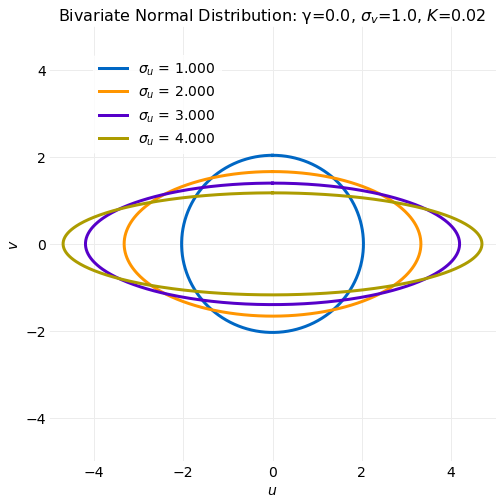
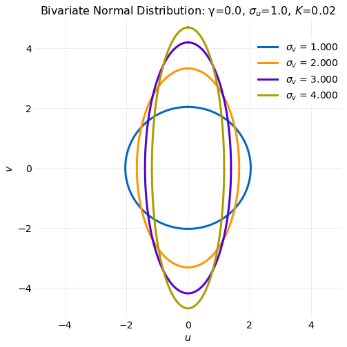
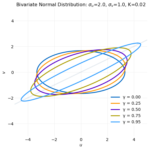
To get a sense of how the contour shape varies with the distribution parameters the following two
plots scan a range of σv/σu with
γ=0 to illustrate the
limits σv/σu→0 and
σv/σu→∞.
This result agrees with the expectation obtained in the previous analysis.
The σv/σu→0 series of contours approaches the u axis and
the σv/σu→∞ contours approach the
v axis.
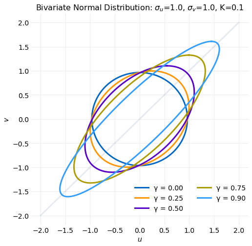
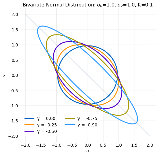
The next two plots illustrate the limit γ→1 and
γ→−1 with σv/σu=1.
The γ→1 plot is converging to the line
v=u and the γ→−1 plot to the line
v=−u as described in the previous section.
Note that as γ
approaches the limit the semi-major axis of the contour increases along
the appropriate limiting line without any rotation of the contour.
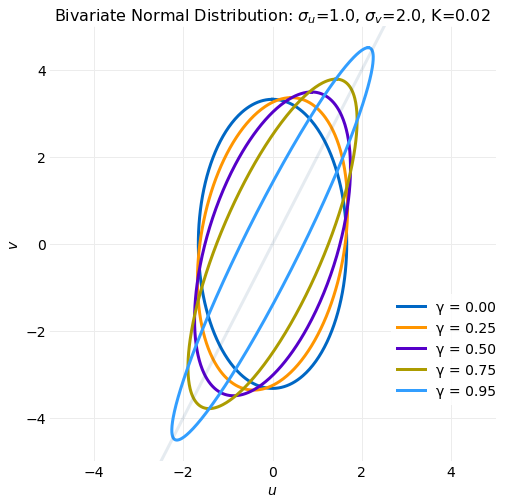
The final two plots also look at the γ→1 limit but this time
the first plot has σv/σu=0.5 and the second
σv/σu=2. The first is converging to the line
v=u/2 and the second converges to the
line v=2u in agreement with the previous analysis. The behavior of the
contour as the limit is approached is more interesting since the ellipse has to rotate to reach the limit.
This is caused by the γ=0 contour also being an ellipse which
introduces and asymmetry that must be eliminated in the limit. If the γ=0
contour were a symmetric circle no initial asymmetry need to be erased.
Coordinate Transformation
In this section contours of constant u and v
are plotted in the (x,y) coordinate system using equation
(6) to understand how the transform distorts area elements as the
distribution parameters are varied.
Contours of constant u=Cu in (x,y)
coordinates are defined by,
Substituting the expression for x into the expression for
y gives,
y=1−γ2−γx+σv1−γ21(Cv−μv),
which is the equation of a line with slope −γ/1−γ2.
First, consider the case γ=0, μu=μv=0
and σu=σv=1 which results in the transform,
xy=Cu=Cv,
and the Jacobian, equation (10), is given by,
∣J∣=σuσv1−γ21=1.
It follows that area elements satisfy,
dxdy=∣J∣dudv=dudv.
Thus, for this particular choice of transform parameters area elements are preserved.
Inspection of the following plot confirms that this is the case since the
transform exactly maps (u,v) coordinates onto (x,y)
coordinates.
The next plot has parameters γ=0 and σu=1
and σv=2. The transform associated this parameter choice is given by,
xy=Cu=21Cv,
with Jacobian,
∣J∣=σuσv1−γ21=21.
Once again the u contours are aligned with lines of constant
x but the v contours are compressed by a
factor of 2 relative to lines of constant y.
If follows that the transform reduces the size of (u,v)
area elements by a factor of 1/2 when transformed, namely,
dxdy=∣J∣dudv=21dudv.
What this is saying is that for an arbitrary area element dudv in the
(u,v) coordinates when transformed to the (x,y)
coordinates the dxdy element has 1/2 the area.
This is seen to be the case in the plot where the area of a (u,v)
rectangle is reduced by a factor of 2.
The final plot considers the impact of correlation on the transform by using the parameters
γ=0.5 and σu=σv=1. The transform corresponding
to this parameter choice is given by,
xy=Cu=(−31x+32Cv),
with Jacobian,
∣J∣=σuσv1−γ21=32.
The u contours are aligned again but now since there is correlation the
v contours are lines with a negative slope so rectangular area elements in
(u,v) are transformed into parallelograms in (x,y)
coordinates. The area of one of the parallelograms is ΔyΔx, where
Δy is the spacing between contours of constant v
and Δx is the spacing between contours of constant u.
Now, from the transform above it is seen that,
ΔxΔy=ΔCu=32ΔCv,
but ΔCu=ΔCv=1, so the area of the parallelogram is given by,
ΔyΔx=32,
which is equal to the Jacobian. It follows that for this choice of parameters the transformation area
elements are increased in size by a factor of 2/3,
dxdy=∣J∣dudv=32dudv.
Conclusions
The Bivariate Normal distribution provides a simple model of correlated random
variables. It is interesting to study because it is modeled as a linear transform of independent
Normal(0,1) random variables that can serve as an introduction to
the concepts used in transformations of multivariate integrals.
Here the background needed to understand transformations of bivariate integrals was developed by starting with a discussion of the interpretation of the vector cross product as an area. This idea was then
applied to the derivation of the Jacobian Matrix for an arbitrary bivariate transformation of
differential area elements. Next, the transformation used to define the Bivariate Normal distribution was
introduced and applied to a distribution of two independent Normal(0,1) random variables. The Jacobian matrix was then computed and the Bivariate Normal PDF derived.
A matrix form of the Bivariate Normal PDF based the covariance matrix was introduced and shown to
be equivalent to the linear transform version first discussed. The covariance matrix form more easily
extends to higher dimensions. The linear transform used to define the Bivariate Normal PDF introduced
five parameters. It was next shown that these parameters are the means,
μu,μv, variance, σu,σv
and correlation coefficient, γ, of the distribution.
The conditional distributions were also discussed.
The change in shape of the distribution as the parameters were varied was then investigated by
evaluating limits for the PDF contours that included γ→0,
γ→±1, σv/σu→1,
σv/σu→0 and
σv/σu→∞. This was followed by numerically investigating the convergence to these limits using a parametric form of the PDF contour equation.
The last topic discussed was the variation of the linear coordinate transformation with the distribution
parameters. It was shown that resulting changes in transformed area elements were accounted for
by the Jacobian.