Rejection Sampling

Rejection Sampling is a method for obtaining samples for a known target probability distribution using samples from some other proposal distribution. It is a more general method than Inverse CDF Sampling which requires distribution to have an invertible CDF. Inverse CDF Sampling transforms a $\textbf{Uniform}(0,\ 1)$ random variable into a random variable with a desired target distribution using the inverted CDF of the target distribution. While, Rejection Sampling is a method for transformation of random variables from arbitrary proposal distributions into a desired target distribution.

The implementation of Rejection Sampling requires the consideration of a target distribution, $f_X(X)$, a proposal distribution, $f_Y(Y)$, and a $\textbf{Uniform}(0,\ 1)$ acceptance probability, $U$, with distribution $f_U(U)=1$. A proposal sample, $Y$, is generated using, $f_Y(Y)$, and independently a uniform acceptance sample, $U$, is generated using $f_U(U)$. A criterion is defined for acceptance of a sample, $X$, to be considered a sample of $f_X(X)$,

$U\ \leq\ \frac{f_X(Y)}{cf_Y(Y)}\ \ \ \ \ (1),$

where, $c$, is chosen to satisfy $0\ \leq\ f_X(Y)/cf_Y(Y)\ \leq\ 1, \ \ \forall\ Y$. If equation $(1)$ is satisfied the proposed sample $Y$ is accepted as a sample of $f_X(X)$ where $X=Y$. If equation $(1)$ is not satisfied $Y$ is discarded.

The acceptance function is defined by,

$h(Y) = \frac{f_X(Y)}{f_Y(Y)}\ \ \ \ \ (2).$

It can be insightful to compare $h(y)$ to $f_X(y)$ when choosing a proposal distribution. If $h(y)$ does not share sufficient mass with $f_X(Y)$ then the choice of $f_Y(Y)$ should be reconsidered.

The Rejection Sampling algorithm can be summarized in the following steps that are repeated for the generation of each sample,

1. Generate a sample $Y \sim f_Y(Y)$.
2. Generate a sample $U\sim\textbf{Uniform}(0,\ 1)$ independent of $Y$.
3. If equation $(1)$ is satisfied then $X=Y$ is accepted as a sample of $f_X(X)$. If equation $(1)$ is not satisfied then $Y$ is discarded.

Theory

To prove that Rejection Sampling works it must be shown that, $P\left[Y\ \leq\ y\ |\ U\ \leq\ \frac{f_X(Y)}{cf_Y(Y)}\right]=F_X(y)\ \ \ \ \ (3),$

where $F_X(y)$ is the CDF for $f_X(y)$, $F_X(y) = \int_{-\infty}^{y} f_X(w)dw.$

To prove equation $(2)$ a couple of intermediate steps are required. First, The joint distribution of $U$ and $Y$ containing the acceptance constraint will be shown to be,

$P\left[U\ \leq\ \frac{f_X(Y)}{cf_Y(Y)},\ Y\ \leq\ y\right] = \frac{F_X(y)}{c}\ \ \ \ \ (4).$

Since the Rejection Sampling algorithm as described in the previous section assumes that $Y$ and $U$ are independent random variables, $f_{YU}(Y, U)\ =\ f_Y(Y)f_U(U)\ = f_Y(Y).$ It follows that,

$\begin{aligned} P\left[U\ \leq\ \frac{f_X(Y)}{cf_Y(Y)},\ Y\ \leq y\right] &= \int_{-\infty}^{y}\int_{0}^{f_X(w)/cf_Y(w)} f_{YU}(w, u) du dw\\ &= \int_{-\infty}^{y}\int_{0}^{f_X(w)/cf_Y(w)} f_Y(w) du dw \\ &= \int_{-\infty}^{y} f_Y(w) \int_{0}^{f_X(w)/cf_Y(w)} du dw \\ &= \int_{-\infty}^{y} f_Y(w) \frac{f_X(w)}{cf_Y(w)} dw \\ &= \frac{1}{c}\int_{-\infty}^y f_X(w) dw \\ &= \frac{F_X(y)}{c}, \\ \end{aligned}$

Next, it will be shown that, $P\left[U\ \leq\ \frac{f_X(Y)}{cf_Y(Y)}\right] = \frac{1}{c}\ \ \ \ \ (5).$

This result follows from equation $(4)$ by taking the limit $y\to\infty$ and noting that, $\int_{-\infty}^{\infty} f_X(y) dy = 1$.

$\begin{aligned} P\left[U\ \leq\ \frac{f_X(Y)}{cf_Y(Y)}\right] &= \int_{-\infty}^{\infty}\int_{0}^{f_X(w)/cf_Y(w)} f_{YU}(w, u) du dw\\ &= \frac{1}{c}\int_{-\infty}^{\infty} f_X(w) dw \\ &= \frac{1}{c} \end{aligned}$

Finally, equation $(3)$ can be proven, using the definition of Conditional Probability, equation $(4)$ and equation $(5)$,

$\begin{aligned} P\left[Y\ \leq\ y\ |\ U\ \leq\ \frac{f_X(Y)}{cf_Y(Y)}\right] &= \frac{P\left[U\ \leq\ \frac{f_X(Y)}{cf_Y(Y)},\ Y \leq y\right]}{P\left[U\ \leq\ \frac{f_X(Y)}{cf_Y(Y)}\right]}\\ &=\frac{F_X(y)}{c}\frac{1}{1/c}\\ &=F_X(y) \end{aligned}$

Implementation

An implementation in Python of the Rejection Sampling algorithm is listed below,

def rejection_sample(h, y_samples, c):
    nsamples = len(y_samples)
    u = numpy.random.rand(nsamples)
    accepted_mask = (u <= h(y_samples) / c)
    return y_samples[accepted_mask]

The above function rejection_sample(h, y_samples, c) takes three arguments as input which are described in the table below.

Argument	Description
h	The acceptance function. Defined by $h(Y)=f_X(Y)/f_Y(Y)$.
y_samples	Array of samples of $Y$ generated using $f_Y(Y)$.
c	A constant chosen so $0\ \leq\ h(Y)/c\ \leq\ 1, \ \ \forall\ Y$

The execution of rejection_sample(h, y_samples, c) begins by generating an appropriate number of acceptance variable samples, $U$, and then determines which satisfy the acceptance criterion specified by equation (1). The accepted samples are then returned.

Examples

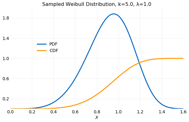
Consider the $\textbf{Weibull}$ Distribution. The PDF is given by,

$f_X(x; k, \lambda) = \begin{cases} \frac{k}{\lambda}\left(\frac{x}{\lambda} \right)^{k-1} e^{-\left(x/\lambda\right)^k} & x\ \geq\ 0 \\ 0 & x < 0 \end{cases} \ \ \ \ \ (4),$

where $k\ >\ 0$ is the shape parameter and $\lambda\ >\ 0$ the scale parameter. The CDF is given by,

$F_X(x; k, \lambda) = \begin{cases} 1-e^{\left(\frac{-x}{\lambda}\right)^k } & x \geq 0 \\ 0 & x < 0. \end{cases}$

The first and second moments are,

$\begin{aligned} \mu & = \lambda\Gamma\left(1+\frac{1}{k}\right) \\ \sigma^2 & = \lambda^2\left[\Gamma\left(1+\frac{2}{k}\right)-\left(\Gamma\left(1+\frac{1}{k}\right)\right)^2\right] \end{aligned} \ \ \ \ \ (5),$

where $\Gamma(x)$ is the Gamma function. In the examples described here it will be assumed that $k=5.0$ and $\lambda=1.0$. The plot below shows the PDF and CDF using these values.

The following sections will compare the performance of generating $\textbf{Weibull}$ samples using both $\textbf{Uniform}(0,\ m)$ and $\textbf{Normal}(\mu,\ \sigma)$ proposal distributions.

Uniform Proposal Distribution

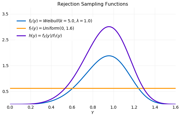
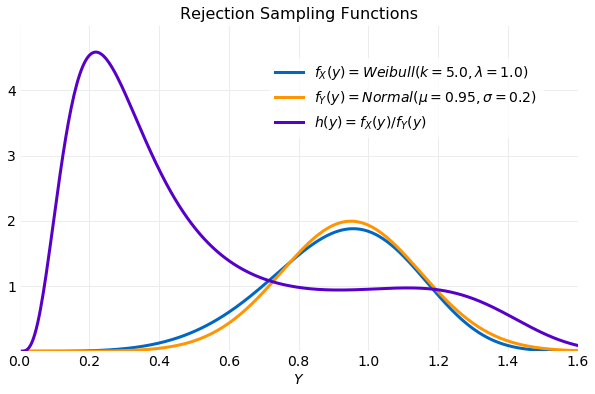
Here a $\textbf{Uniform}(0,\ m)$ proposal distribution will be used to generate samples for the $\textbf{Weibull}$ distribution $(4)$. It provides a simple and illustrative example of the algorithm. The following plot shows the target distribution $f_X(y)$, the proposal distribution $f_Y(y)$ and the acceptance function $h(y)=f_X(y)/f_Y(y)$ used in this example. The uniform proposal distribution requires that a bound be placed on the proposal samples, which will be assumed to be $m=1.6$. Since the proposal distribution is constant the acceptance function, $h(y)$, will be a constant multiple of the target distribution. This is illustrated in the plot below.

The Python code used to generate the samples using rejection_sample(h, y_samples, c) is listed below.

weibull_pdf = lambda v: (k/λ)*(v/λ)**(k-1)*numpy.exp(-(v/λ)**k)

k = 5.0
λ = 1.0

xmax = 1.6
ymax = 2.0
nsamples = 100000

y_samples = numpy.random.rand(nsamples) * xmax
samples = rejection_sample(weibull_pdf, y_samples, ymax)

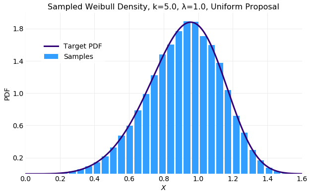
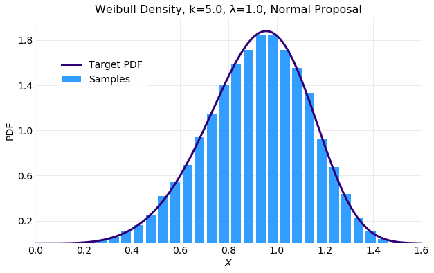
The following plot compares the histogram computed form the generated samples with the target distribution $(4)$. The fit is acceptable.

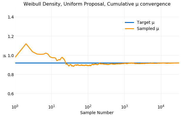
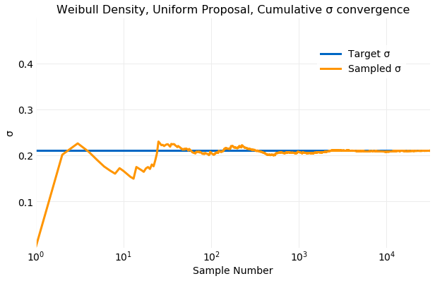
The next two plots illustrate convergence of the sample mean, $\mu$, and standard deviation, $\sigma$, by comparing the cumulative sums computed from the samples to target distribution values computed from equation $(5)$. The convergence of the sampled $\mu$ is quite rapid. Within only $10^2$ samples $\mu$ computed form the samples is very close the the target value and by $10^4$ samples the two values are indistinguishable. The convergence of the sampled $\sigma$ to the target value is not as rapid as the convergence of the sampled $\mu$ but is still quick. By $10^4$ samples the two values are near indistinguishable.

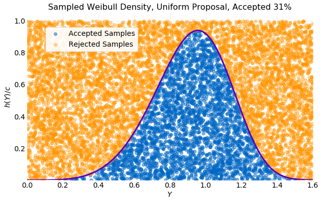
Even though $10^5$ proposal samples were generated not all were accepted. The plot below provides insight into the efficiency of the algorithm. In the plot the generated pairs of acceptance probability $U$ and sample proposal $Y$ are plotted with $U$ on the vertical axis and $Y$ on the horizontal axis. Also, shown is the scaled acceptance function $h(Y)/c$. If $U\ >\ h(Y)/c$ the sample is rejected and colored orange in the plot and if $U\ \leq\ h(Y)/c$ the sample is accepted, $X=Y$ and colored blue. Only $31\%$ of the generated samples were accepted.

To improve the acceptance percentage of proposed samples a different proposal distribution must be considered. In the plot above it is seen that the $\textbf{Uniform}(0,\ 1.6)$ proposal distribution uniformly samples the space enclosed by the rectangle it defines without consideration for the shape of the target distribution. The acceptance percentage will be determined by the ratio of the target distribution area enclosed by the proposal distribution and the proposal distribution area. As the target distribution becomes sharp the acceptance percentage will decrease. A proposal distribution that samples the area under $h(Y)/c$ efficiently will have a higher acceptance percentage. It should be kept in mind that rejection of proposal samples is required for the algorithm to work. If no proposal samples are rejected the proposal and target distributions will be equivalent.

Normal Proposal Distribution

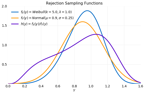
In this section a sampler using a $\textbf{Normal}(\mu,\ \sigma)$ proposal distribution and target $\textbf{Weibull}$ distribution is discussed. A $\textbf{Normal}$ proposal distribution has advantages over the $\textbf{Uniform}(0,\ m)$ distribution discussed in the previous section. First, it can provide unbounded samples, while a uniform proposal requires specifying bounds on the samples. Second, it is a closer approximation to the target distribution so it should provide samples that are accepted with greater frequency. A disadvantage of the $\textbf{Normal}$ proposal distribution is that it requires specification of $\mu$ and $\sigma$. If these parameters are the slightest off the performance of the sampler will be severely degraded. To learn this lesson the first attempt will assume values for both the parameters that closely match the target distribution. The following plot compares the $f_X(y)$, the proposal distribution $f_Y(y)$ and the acceptance function $h(y)$. There is a large peak in $h(y)$ to right caused by the more rapid increase of the $\textbf{Weibull}$ distribution relative to the $\textbf{Normal}$ distribution with the result that most of its mass is not aligned with the target distribution.

The Python code used to generate the samples using rejection_sample(h, y_samples, c) is listed below.

weibull_pdf = lambda v: (k/λ)*(v/λ)**(k-1)*numpy.exp(-(v/λ)**k)

def normal(μ, σ):
    def f(x):
        ε = (x - μ)**2/(2.0*σ**2)
        return numpy.exp(-ε)/numpy.sqrt(2.0*numpy.pi*σ**2)
    return f

k = 5.0
λ = 1.0

σ = 0.2
μ = 0.95

xmax = 1.6
nsamples = 100000

y_samples = numpy.random.normal(μ, σ, nsamples)
ymax = h(x_values).max()
h = lambda x: weibull_pdf(x) / normal(μ, σ)(x)

samples = rejection_sample(h, y_samples, ymax)

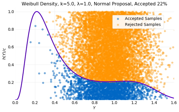
The first of the following plots compares the histogram computed from the generated samples with the target distribution $(4)$ and the second illustrates which proposal samples were accepted. The histogram fit is good but only $23\%$ of the samples were accepted which is worse than the result obtained with the uniform proposal previously discussed.

In an attempt to improve the acceptance rate $\mu$ of the proposal distribution is decreased slightly and $\sigma$ is increased. The result is shown in the next plot. The proposal distribution now covers the target distribution tails. The acceptance function, $h(Y)$, now has its peak inside the target distribution with significant overlap of mass.

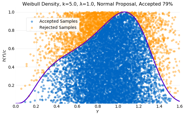
The result is much improved. In the plot below it is seen that the percentage of accepted samples has increased to $79\%$.

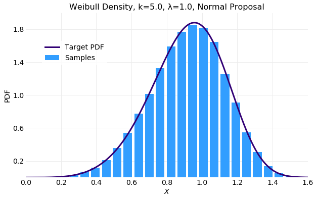
The first of the plots below compares the histogram computed from generated samples with the target distribution $(4)$ and next two compare the cumulative values of $\mu$ and $\sigma$ computed from the generated samples with the target distribution values from equation $(5)$. The histogram is the best fit of the examples discussed here and convergence of the sampled $\mu$ and $\sigma$ occurs in about $10^3$ samples.

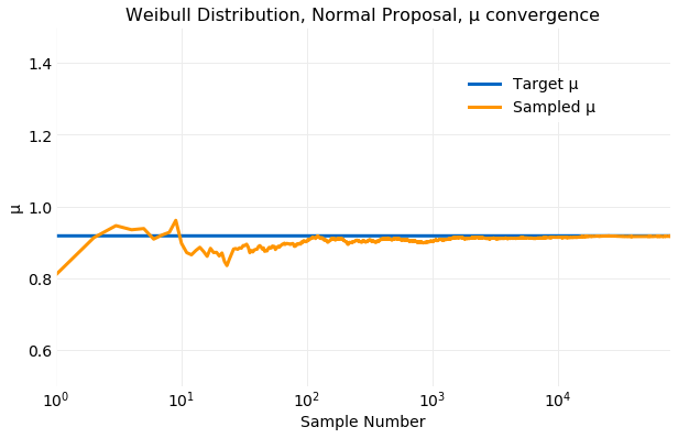
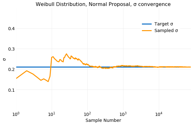
Sampling the $\textbf{Weibull}$ distribution with a $\textbf{Normal}$ proposal distribution can produce a better result than a uniform distribution but care must be exercised in selecting the $\textbf{Normal}$ distribution parameters. Some choices can produce inferior results. Analysis of the the acceptance function $(2)$ can provide guidance in parameter selection.

Conclusions

Rejection Sampling provides a general method for generation of samples for a known target distribution by rejecting or accepting samples from a known proposal distribution sampler. It was analytically proven that if proposal samples are accepted with a probability defined by equation $(1)$ the accepted samples have the desired target distribution. An algorithm implementation was discussed and used in examples where its performance in producing samples with a desired target distribution for several different proposal distributions was investigated. Mean and standard deviations computed from generated samples converged to the target distribution values in $O(10^3)$ samples.for both the discrete and continuous cases. It was shown that the performance of the algorithm can vary significantly with chosen parameter values for the proposal distribution. A criteria for evaluating the expected performance of a proposal distribution using the acceptance function, defined by equation $(2)$, was suggested. Performance was shown to improve if the acceptance function has significant overlap with the proposal distribution.