Discrete State Markov Chain Equilibrium

A Markov Chain is a sequence of states where transitions between states occur ordered in time with the probability of transition depending only on the previous state. Here the states will be assumed a discrete finite set and time a discrete unbounded set. If the set of states is given by $\{x_1,\ x_2,\ldots,\ x_N\}$ the probability that the process will be in state $x_i$ at time $t$ is denoted by $P(X_t=x_i)$, referred to as the distribution. Markov Chain equilibrium is defined by $\lim_{t\to\infty}P(X_t=x_i)\ <\ \infty$, that is, as time advances
$P(X_t=x_i)$ becomes independent of time. Here a solution for this limit is discussed and illustrated with examples.

Model

The Markov Chain model is constructed from the set of states $\{x_1,\ x_2,\ldots,\ x_N\}$ ordered in time. The process starts at time $t=0$ with state $X_0=x_i$. At the next step, $t=1$, the process will assume a state $X_1=x_j$ with probability $P(X_1=x_j|X_0=x_i)$ since it will depend on the previous state $x_0$ as defined for a Markov Process. At the next time step $t=2$ the process state will be $X_2=x_k$ with probability, $P(X_2=x_k|X_0=x_i, X_1=x_j)=P(X_2=x_k|X_1=x_j),$ since by definition the probability of state transition depends only upon the state at the previous time step. For an arbitrary time the transition from a state $X_{t}=x_j$ to a state $X_{t+1}=x_j$ will occur with probability, $P(X_{t+1}=x_j|X_t=x_i)$ that is independent of $t$. Transition probabilities have the form of a matrix,

$P_{ij} = P(X_{t+1}=x_j|X_t=x_i).$

$P$ will be an $N\times N$ matrix where $N$ is determined by the number of possible states. Each row represents the Markov Chain transition probability from that state at time $t$ and the columns the values at $t+1$. It follows that, $\begin{gathered} \sum_{j=1}^{N}P_{ij} = 1\\ P_{ij}\ \geq\ 0 \end{gathered} \ \ \ \ \ (1).$

Equation $(1)$ is the definition of a Stochastic Matrix.

The transition probability for a single step in the Markov Process is defined by $P$. The transition probability across two time steps can be obtained with use of the Law of Total Probability, $\begin{aligned} P(X_{t+2}=x_j|X_t=x_i) &= \sum_{k=1}^{N} P(X_{t+2}=x_j | X_{t}=x_i, X_{t+1}=x_k)P(X_{t+1}=x_k | X_{t}=x_i) \\ &= \sum_{k=1}^{N} P(X_{t+2}=x_j | X_{t+1}=x_k)P(X_{t+1}=x_k | X_{t}=x_i) \\ &= \sum_{k=1}^{N} P_{kj}P_{ik} \\ &= \sum_{k=1}^{N} P_{ik}P_{kj} \\ &= {(P^2)}_{ij}, \end{aligned}$

where the last step follows from the definition of matrix multiplication. It is straight forward but tedious to use Mathematical Induction to extend the previous result to the case of an arbitrary time difference, $\tau$, $P(X_{t+\tau}=x_j|X_t=x_i) = {(P^{\tau})}_{ij}\ \ \ \ \ (2).$

It should be noted that since ${(P^{\tau})}_{ij}$ is a transition probability it must satisfy,

$\begin{gathered} \sum_{j=1}^{N} {(P^{\tau})}_{ij}\ =\ 1 \\ {(P^{\tau})}_{ij}\ \geq\ 0 \end{gathered} \ \ \ \ \ (3).$

To determine the equilibrium solution of the distribution of states, $\{x_1,\ x_2,\ldots,\ x_N\}$, the distribution time variability must be determined. Begin by considering an arbitrary distribution at $t=0$, which can be written as a column vector, $\pi = \begin{pmatrix} \pi_1 \\ \pi_2 \\ \vdots \\ \pi_N \end{pmatrix} = \begin{pmatrix} P(X_0=x_1) \\ P(X_0=x_2) \\ \vdots \\ P(X_0=x_N) \end{pmatrix},$

since it is a probability distribution $\pi_i$ must satisfy, $\begin{gathered} \sum_{i=1}^{N} \pi_i\ =\ 1\\ \pi_i\ \geq \ 0 \end{gathered} \ \ \ \ \ (4).$

The distribution after the first step is given by, $\begin{aligned} P(X_1=x_j) &= \sum_{i=1}^{N} P(X_1=x_j|X_0=x_i)P(X_0=x_i) \\ &= \sum_{i=1}^{N} P_{ij}\pi_{i} \\ &= \sum_{i=1}^{N} \pi_{i}P_{ij} \\ &= {(\pi^{T}P)}_{j}, \end{aligned}$

where $\pi^T$ is the transpose of $\pi$. Similarly, the distribution after the second step is, $\begin{aligned} P(X_2=x_j) &= \sum_{i=1}^{N} P(X_2=x_j|X_1=x_i)P(X_1=x_i) \\ &= \sum_{i=1}^{N} P_{ij}{(\pi^{T}P)}_{i} \\ &= \sum_{i=1}^{N} P_{ij}\sum_{k=1}^{N} \pi_{k}P_{ki} \\ &= \sum_{k=1}^{N} \pi_{k} \sum_{i=1}^{N} P_{ij}P_{ki} \\ &= \sum_{k=1}^{N} \pi_{k} \sum_{i=1}^{N} P_{ki}P_{ij} \\ &= \sum_{k=1}^{N} \pi_{k} {(P^2)}_{kj} \\ &= {(\pi^{T}P^2)}_{j}, \end{aligned}$

A pattern is clearly developing. Mathematical Induction can be used to prove the distribution at an arbitrary time $t$ is given by, $P(X_t=x_j) = {(\pi^{T}P^t)}_{j}$

or as a column vector,

$\pi_{t}^{T} = \pi^{T}P^t\ \ \ \ \ (5).$

Where $\pi$ and $\pi_t$ are the initial distribution and the distribution after $t$ steps respectively.

Equilibrium Transition Matrix

The probability of transitioning between two states $x_i$ and $x_j$ in $t$ time steps was previously shown to be stochastic matrix $P^t$ constrained by equation $(3)$. The equilibrium transition matrix is defined by, $P^{E} = \lim_{t\to\infty}P^{t}.$ This limit can be determined using Matrix Diagonalization. The following sections will use diagonalization to construct a form of $P^{t}$ that will easily allow evaluation equilibrium limit.

Eigenvectors and Eigenvalues of the Transition Matrix

Matrix Diagonalization requires evaluation of eigenvalues and eigenvectors, which are defined by the solutions to the equation, $Pv = \lambda v\ \ \ \ \ (6),$ where $v$ is the eigenvector and $\lambda$ eigenvalue. From equation $(6)$ it follows, $\begin{aligned} P^{t}v &= P^{t-1}(Pv)\\ &=P^{t-1}\lambda v\\ &=P^{t-2}(Pv)\lambda\\ &=P^{t-2}\lambda^{2}v \\ &\vdots\\ &=(Pv)\lambda^{t-1}\\ &=\lambda^{t}v. \end{aligned}$

Since $P^t$ is a stochastic matrix it satisfies equation $(3)$. As a result of these constraints the limit $t\to\infty$ requires, $\lim_{t\to\infty}P^{t}=\lim_{t\to\infty}\lambda^{t}v\ \leq\ \infty.$

It follows that $\lambda\ \leq\ 1$. Next, it will be shown that $\lambda_1=1$ and that a column vector of $1's$ with $N$ rows, $V_1 = \begin{pmatrix} 1 \\ 1 \\ \vdots \\ 1 \end{pmatrix}\ \ \ \ \ (7),$ are eigenvalue and eigenvector solutions of equation $(6)$, $\begin{pmatrix} P_{11} & P_{12} & \cdots & P_{1N} \\ P_{21} & P_{22} & \cdots & P_{2N} \\ \vdots & \vdots & \ddots & \vdots \\ P_{N1} & P_{N2} & \cdots & P_{NN} \end{pmatrix} \begin{pmatrix} 1 \\ 1 \\ \vdots \\ 1 \end{pmatrix} = \begin{pmatrix} \sum_{j=1}^{N}P_{1j} \\ \sum_{j=1}^{N}P_{2j} \\ \vdots \\ \sum_{j=1}^{N}P_{Nj} \end{pmatrix} = \begin{pmatrix} 1 \\ 1 \\ \vdots \\ 1 \end{pmatrix} =\lambda_1 V_1,$

where use was made of the stochastic matrix condition from equation $(1)$, namely, $\sum_{j=1}^{N}P_{ij}=1$.

To go further a result from the Perron-Frobenius Theorem is needed. This theorem states that a stochastic matrix will have a largest eigenvalue with multiplicity 1. Here all eigenvalues will satisfy $\lambda_1=1 \ >\ \mid{\lambda_i}\mid,\ \forall\ 1\ <\ i\ \leq\ N$.

Denote the eigenvector $V_j$ by the column vector, $V_j = \begin{pmatrix} v_{1j} \\ v_{2j} \\ \vdots \\ v_{Nj} \end{pmatrix},$

and let $V$ be the matrix with columns that are the eigenvectors of $P$ with $V_1$ from equation $(7)$ in the first column, $V= \begin{pmatrix} 1 & v_{12} & \cdots & v_{1N} \\ 1 & v_{22} & \cdots & v_{2N} \\ \vdots & \vdots & \ddots & \vdots \\ 1 & v_{N2} & \cdots & v_{NN} \end{pmatrix}.$

Assume that $V$ is invertible and denote the inverse by,

$V^{-1}= \begin{pmatrix} v^{-1}_{11} & v^{-1}_{12} & \cdots & v^{-1}_{1N} \\ v^{-1}_{21} & v^{-1}_{22} & \cdots & v^{-1}_{2N} \\ \vdots & \vdots & \ddots & \vdots \\ v^{-1}_{N1} & v^{-1}_{N2} & \cdots & v^{-1}_{NN} \end{pmatrix}\ \ \ \ \ (8).$

If the identity matrix is represented by $I$ then $VV^{-1} = I$. Let $\Lambda$ be a diagonal matrix constructed from the eigenvalues of $P$ using $\lambda_1=1$,

$\Lambda = \begin{pmatrix} 1 & 0 & \cdots & 0 \\ 0 & \lambda_2 & \cdots & 0 \\ \vdots & \vdots & \ddots & \vdots \\ 0 & 0 & \cdots & \lambda_N \end{pmatrix}.$

Sufficient information about the eigenvalues and eigenvectors has been obtained to prove some very general results for Markov Chains. The following section will work through the equilibrium limit using the using these results to construct a diagonalized representation of the matrix.

Diagonalization of Transition Matrix

Using the results obtained in the previous section the diagonalized form of the transition matrix is given by,

$P = V\Lambda V^{-1},$

Using this representation of $P$ an expression for $P^t$ is obtained, $\begin{aligned} P^{t} &= P^{t-1}V\Lambda V^{-1} \\ &= P^{t-2}V\Lambda V^{-1}V\Lambda V^{-1} \\ &= P^{t-2}V\Lambda^2 V^{-1}\\ &\vdots \\ &= PV\Lambda^{t-1} V^{-1} \\ &= V\Lambda^{t}V^{-1} \end{aligned}$

Evaluation of $\Lambda^{t}$ is straight forward,

$\Lambda^t = \begin{pmatrix} 1 & 0 & \cdots & 0 \\ 0 & \lambda_2^t & \cdots & 0 \\ \vdots & \vdots & \ddots & \vdots \\ 0 & 0 & \cdots & \lambda_N^t \end{pmatrix}.$

Since $\mid{\lambda_i}\mid\ <\ 1,\ \forall\ 1\ <\ i\ \leq\ N$ in the limit $t\to\infty$ it is seen that, $\Lambda^{E} = \lim_{t\to\infty} \Lambda^t = \lim_{t\to\infty} \begin{pmatrix} 1 & 0 & \cdots & 0 \\ 0 & \lambda_2^t & \cdots & 0 \\ \vdots & \vdots & \ddots & \vdots \\ 0 & 0 & \cdots & \lambda_N^t \end{pmatrix} = \begin{pmatrix} 1 & 0 & \cdots & 0 \\ 0 & 0 & \cdots & 0 \\ \vdots & \vdots & \ddots & \vdots \\ 0 & 0 & \cdots & 0 \end{pmatrix},$

so, $P^{E} = \lim_{t\to\infty} P^{t} = \lim_{t\to\infty} V\Lambda^{t} V^{-1} = V\Lambda^{E}V^{-1}.$

Evaluation of the first two terms on the righthand side gives,

$V\Lambda^{E} = \begin{pmatrix} 1 & v_{12} & \cdots & v_{1N} \\ 1 & v_{22} & \cdots & v_{2N} \\ \vdots & \vdots & \ddots & \vdots \\ 1 & v_{N2} & \cdots & v_{NN} \end{pmatrix} \begin{pmatrix} 1 & 0 & \cdots & 0 \\ 0 & 0 & \cdots & 0 \\ \vdots & \vdots & \ddots & \vdots \\ 0 & 0 & \cdots & 0 \end{pmatrix} = \begin{pmatrix} 1 & 0 & \cdots & 0 \\ 1 & 0 & \cdots & 0 \\ \vdots & \vdots & \ddots & \vdots \\ 1 & 0 & \cdots & 0 \end{pmatrix}.$

It follows that, $V\Lambda^{E} V^{-1} = \begin{pmatrix} 1 & 0 & \cdots & 0 \\ 1 & 0 & \cdots & 0 \\ \vdots & \vdots & \ddots & \vdots \\ 1 & 0 & \cdots & 0 \end{pmatrix} \begin{pmatrix} v^{-1}_{11} & v^{-1}_{12} & \cdots & v^{-1}_{1N} \\ v^{-1}_{21} & v^{-1}_{22} & \cdots & v^{-1}_{2N} \\ \vdots & \vdots & \ddots & \vdots \\ v^{-1}_{N1} & v^{-1}_{N2} & \cdots & v^{-1}_{NN} \end{pmatrix} = \begin{pmatrix} v^{-1}_{11} & v^{-1}_{12} & \cdots & v^{-1}_{1N} \\ v^{-1}_{11} & v^{-1}_{12} & \cdots & v^{-1}_{1N} \\ \vdots & \vdots & \ddots & \vdots \\ v^{-1}_{11} & v^{-1}_{12} & \cdots & v^{-1}_{1N} \end{pmatrix}.$

Finally, the equilibrium transition matrix is given by, $P^{E} = V\Lambda^{E} V^{-1} = \begin{pmatrix} v^{-1}_{11} & v^{-1}_{12} & \cdots & v^{-1}_{1N} \\ v^{-1}_{11} & v^{-1}_{12} & \cdots & v^{-1}_{1N} \\ \vdots & \vdots & \ddots & \vdots \\ v^{-1}_{11} & v^{-1}_{12} & \cdots & v^{-1}_{1N} \end{pmatrix}\ \ \ \ \ (9).$

The rows of $P^{E}$ are identical and given by the first row of the inverse of the matrix of eigenvectors, $V^{-1}$, from equation $(8)$. This row is a consequence of the location of the $\lambda=1$ eigenvalue and eigenvector in $\Lambda$ and $V$ respectively. Since $P^{E}$ is a transition matrix,

$\begin{gathered} \sum_{j=1}^{N} v_{ij}^{-1}\ =\ 1\\ v_{ij}^{-1}\ \geq \ 0. \end{gathered}$

Equilibrium Distribution

The equilibrium distribution is defined by a solution to equation $(5)$ that is independent of time.

$\pi^{T} = \pi^{T}P^t\ \ \ \ \ (10).$

Consider a distribution $\pi_{E}$ that satisfies, $\pi_{E}^{T} = \pi_{E}^{T}P\ \ \ \ \ (11).$

It is easy to show that $\pi_{E}$ is an equilibrium solution by substituting it into equation $(10)$. $\begin{aligned} \pi_{E}^{T} &= \pi_{E}^{T}P^t \\ &= (\pi_{E}^{T}P)P^{t-1} \\ &= \pi_{E}^{T}P^{t-1} \\ &= \pi_{E}^{T}P^{t-2} \\ &\vdots \\ &= \pi_{E}^{T}P \\ &= \pi_{E}^{T}. \end{aligned}$

Relationship Between Equilibrium Distribution and Transition Matrix

To determine the relationship between $\pi_E$ and $P^{E}$, begin by considering an arbitrary initial distribution states with $N$ elements, $\pi = \begin{pmatrix} \pi_{1} \\ \pi_{2} \\ \vdots \\ \pi_{N} \end{pmatrix},$

where,

$\begin{gathered} \sum_{j=1}^{N}\pi_{j} = 1\\ \pi_{j}\ \geq\ 0 \end{gathered}.$

The distribution when the Markov Chain has had sufficient time to reach equilibrium will be given by, $\begin{aligned} \pi^{T}P^{E} &= \begin{pmatrix} \pi_{1} & \pi_{2} & \cdots & \pi_{N} \end{pmatrix} \begin{pmatrix} v^{-1}_{11} & v^{-1}_{12} & \cdots & v^{-1}_{1N} \\ v^{-1}_{11} & v^{-1}_{12} & \cdots & v^{-1}_{1N} \\ \vdots & \vdots & \ddots & \vdots \\ v^{-1}_{11} & v^{-1}_{12} & \cdots & v^{-1}_{1N} \end{pmatrix} \\ &= \begin{pmatrix} v^{-1}_{11}\sum_{j=1}^{N} \pi_{j} & v^{-1}_{12}\sum_{j=1}^{N} \pi_{j} & \cdots & v^{-1}_{1N}\sum_{j=1}^{N} \pi_{j} \end{pmatrix}, \end{aligned}$

since, $\sum_{j=1}^{N} \pi_{j} = 1$,

$\pi^{T}P^{E} = \begin{pmatrix} v^{-1}_{11} & v^{-1}_{12} & \cdots & v^{-1}_{1N} \end{pmatrix}.$

Thus any initial distribution $\pi$ will after sufficient time approach the distribution above. It follows that it will be the solution of equation $(11)$ which defines the equilibrium distribution,

$\pi_E = \begin{pmatrix} v^{-1}_{11} \\ v^{-1}_{12} \\ \vdots \\ v^{-1}_{1N} \end{pmatrix}.$

Solution of Equilibrium Equation

An equation for the equilibrium distribution, $\pi_{E}$, can be obtained from equation $(11)$, $\pi^{T}_E\left(P - I\right) = 0\ \ \ \ \ (12),$ where $I$ is the identity matrix. Equation $(12)$ alone is insufficient to obtain a unique solution since the system of linear equations it defines is Linearly Dependent. In a linearly dependent system of equations some equations are the result of linear operations on the others. It is straight forward to show that one of the equations defined by $(12)$ can be eliminated by summing the other equations and multiplying by $-1$. If the equations were linearly independent the only solution would be the trivial zero solution, ${\left( \pi^{T}_E \right)}_{i}\ =\ 0,\ \forall\ i$. A unique solution to $(12)$ is obtained by including the normalization constraint, $\sum_{j=1}^{N} {\left( \pi_{E}^{T} \right)}_{j} = 1.$ The resulting system of equations to be solved is given by, $\pi_{E}^{T} \begin{pmatrix} {P_{11} - 1} & P_{12} & \cdots & P_{1N} & 1 \\ P_{21} & {P_{22} -1} & \cdots & P_{2N} & 1 \\ \vdots & \vdots & \ddots & \vdots & \vdots\\ P_{N1} & P_{N2} & \cdots & {P_{NN} - 1} & 1 \\ \end{pmatrix} = \begin{pmatrix} 0 & 0 & 0 & 0 & 1 \end{pmatrix}\ \ \ \ \ (13).$

Example

Consider the Markov Chain defined by the transition matrix, $P = \begin{pmatrix} 0.0 & 0.9 & 0.1 & 0.0 \\ 0.8 & 0.1 & 0.0 & 0.1 \\ 0.0 & 0.5 & 0.3 & 0.2 \\ 0.1 & 0.0 & 0.0 & 0.9 \end{pmatrix}\ \ \ \ \ (14).$ The state transition diagram below provides a graphical representation of $P$.

Convergence to Equilibrium

Relaxation of both the transition matrix and distribution to their equilibrium values is easily demonstrated with the few lines of Python executed within ipython.

In [1]: import numpy
In [2]: t = [[0.0, 0.9, 0.1, 0.0],
   ...:      [0.8, 0.1, 0.0, 0.1],
   ...:      [0.0, 0.5, 0.3, 0.2],
   ...:      [0.1, 0.0, 0.0, 0.9]]
In [3]: p = numpy.matrix(t)
In [4]: p**100
Out[4]:
matrix([[0.27876106, 0.30088496, 0.03982301, 0.38053097],
        [0.27876106, 0.30088496, 0.03982301, 0.38053097],
        [0.27876106, 0.30088496, 0.03982301, 0.38053097],
        [0.27876106, 0.30088495, 0.03982301, 0.38053098]])

Here the transition matrix from the initial state to states $100$ time steps in the future is computed using equation $(2)$. The result obtained has identical rows as obtained in equation $(9)$. $P^{100} = \begin{pmatrix} 0.27876106 & 0.30088496 & 0.03982301 & 0.38053097 \\ 0.27876106 & 0.30088496 & 0.03982301 & 0.38053097 \\ 0.27876106 & 0.30088496 & 0.03982301 & 0.38053097 \\ 0.27876106 & 0.30088495 & 0.03982301 & 0.38053098 \end{pmatrix}\ \ \ \ \ (15).$

For an initial distribution $\pi$ the distribution after $100$ time steps is evaluated using,

In [5]: c = [[0.1],
   ...:      [0.5],
   ...:      [0.35],
   ...:      [0.05]]
In [6]: π = numpy.matrix(c)
In [8]: π.T*p**100
Out[8]: matrix([[0.27876106, 0.30088496, 0.03982301, 0.38053097]])

Here an initial distribution is constructed that satisfies $\sum_{i=0}^3 \pi_i = 1$. Then equation $(5)$ is used to compute the distribution after $100$ time steps. The result is that expected from the previous analysis. In the equilibrium limit the distribution is the repeated row of the equilibrium transition matrix, namely,

$\pi_{100} = \begin{pmatrix} 0.27876106 \\ 0.30088496 \\ 0.03982301 \\ 0.38053097 \end{pmatrix}\ \ \ \ \ (16).$

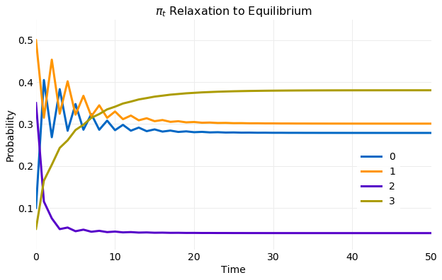
The plot below illustrates the convergence of the distribution from the previous example. In the plot the components of $\pi_t$ from equation $(5)$ are plotted for each time step. The convergence to the limiting value occurs rapidly. Within only $20$ steps $\pi_t$ has reached limiting distribution.

Equilibrium Transition Matrix

In this section the equilibrium limit of the transition matrix is determined for the example Markov Chain shown in equation $(14)$. It was previously shown that this limit is given by equation $(9)$. To evaluate this equation the example transition matrix must be diagonalized. First, the transition matrix eigenvalues and eigenvectors are computed using the numpy linear algebra library.

In [9]: λ, v = numpy.linalg.eig(p)
In [10]: λ
Out[10]: array([-0.77413013,  0.24223905,  1.        ,  0.83189108])
In [11]: v
Out[11]:
matrix([[-0.70411894,  0.02102317,  0.5       , -0.4978592 ],
        [ 0.63959501,  0.11599428,  0.5       , -0.44431454],
        [-0.30555819, -0.99302222,  0.5       , -0.14281543],
        [ 0.04205879, -0.00319617,  0.5       ,  0.73097508]])

It is seen that $\lambda\ =\ 1$ is indeed an eigenvalue, as previously proven and that other eigenvalues have magnitudes less than $1$. This is in agreement with Perron-Frobenius Theorem. The numpy linear algebra library normalizes the eigenvectors and uses the same order for eigenvalues and eigenvector columns. The eigenvector corresponding to $\lambda\ =\ 1$ is in the third column and has all components equal. Eigenvectors are only known to an arbitrary scalar, so the vector of $1's$ used in the previous analysis can be obtained by multiplying the third column by $2$. After obtaining the eigenvalues and eigenvectors equation $(9)$ is evaluated $100$ after time steps and compared with the equilibrium limit.

In [12]: Λ = numpy.diag(λ)
In [13]: V = numpy.matrix(v)
In [14]: Vinv = numpy.linalg.inv(V)
In [15]: Λ_t = Λ**100
In [16]: Λ_t
Out[16]:
array([[7.61022278e-12, 0.00000000e+00, 0.00000000e+00, 0.00000000e+00],
       [0.00000000e+00, 2.65714622e-62, 0.00000000e+00, 0.00000000e+00],
       [0.00000000e+00, 0.00000000e+00, 1.00000000e+00, 0.00000000e+00],
       [0.00000000e+00, 0.00000000e+00, 0.00000000e+00, 1.01542303e-08]])
In [17]: V * Λ_t * Vinv
Out[17]:
matrix([[0.27876106, 0.30088496, 0.03982301, 0.38053097],
        [0.27876106, 0.30088496, 0.03982301, 0.38053097],
        [0.27876106, 0.30088496, 0.03982301, 0.38053097],
        [0.27876106, 0.30088495, 0.03982301, 0.38053098]])

First, the diagonal matrix of eigenvalues, $\Lambda$, is created maintaining the order of $\lambda$. Next, the matrix $V$ is constructed with eigenvectors as columns while also maintaining the order of vectors in $v$. The inverse of $V$ is then computed. $\Lambda^{t}$ can now be computed for $100$ time steps. The result is in agreement with the past effort where the limit $t\to\infty$ was evaluated giving a matrix that contained a $1$ in the $(1,1)$ component corresponding to the position of the $\lambda=1$ component and zeros for all others. Here the eigenvectors are ordered differently but the only nonzero component has the $\lambda=1$ eigenvalue. Finally, equation $(9)$ is evaluated and all rows are identical and equal to $\pi_t$ evaluated at $t=100$, in agreement with the equilibrium limit determined previously and calculations performed in the last section shown in equations $(15)$ and $(16)$.

Equilibrium Distribution

The equilibrium distribution will now be calculated using the system of linear equations defined by equation $(9)$. Below the resulting system of equations for the example distribution in equation $(14)$ is shown.

$\pi_{E}^{T} \begin{pmatrix} -1.0 & 0.9 & 0.1 & 0.0 & 1.0 \\ 0.8 & -0.9 & 0.0 & 0.1 & 1.0 \\ 0.0 & 0.5 & -0.7 & 0.2 & 1.0 \\ 0.1 & 0.0 & 0.0 & -0.1 & 1.0 \end{pmatrix} = \begin{pmatrix} 0.0 & 0.0 & 0.0 & 0.0 & 1.0 \end{pmatrix}$

This system of equations is solved using the least squares method provided by the numpy linear algebra library, which requires the use of the transpose of the above equation. The first line below computes it using equation $(14)$.

In [18]: E = numpy.concatenate((p.T - numpy.eye(4), [numpy.ones(4)]))
In [19]: E
Out[19]:
matrix([[-1. ,  0.8,  0. ,  0.1],
        [ 0.9, -0.9,  0.5,  0. ],
        [ 0.1,  0. , -0.7,  0. ],
        [ 0. ,  0.1,  0.2, -0.1],
        [ 1. ,  1. ,  1. ,  1. ]])
In [20]: πe, _, _, _ = numpy.linalg.lstsq(E, numpy.array([0.0, 0.0, 0.0, 0.0, 1.0]), rcond=None)

In [21]: πe
Out[21]: array([0.27876106, 0.30088496, 0.03982301, 0.38053097])

Next, the equilibrium distribution is evaluated using the least squares method. The result obtained is consistent with previous results shown in equation $(16)$.

Simulation

This section will use a direct simulation of equation $(14)$ to calculate the equilibrium distribution and compare the result to those previously obtained. Below a Python implementation of the calculation is shown.

import numpy

def sample_chain(t, x0, nsample):
    xt = numpy.zeros(nsample, dtype=int)
    xt[0] = x0
    up = numpy.random.rand(nsample)
    cdf = [numpy.cumsum(t[i]) for i in range(4)]
    for t in range(nsample - 1):
        xt[t] = numpy.flatnonzero(cdf[xt[t-1]] >= up[t])[0]
    return xt

# Simulation parameters
π_nsamples = 1000
nsamples = 10000
c = [[0.25],
     [0.25],
     [0.25],
     [0.25]]

# Generate π_nsamples initial state samples
π = numpy.matrix(c)
π_cdf = numpy.cumsum(c)
π_samples = [numpy.flatnonzero(π_cdf >= u)[0] for u in numpy.random.rand(π_nsamples)]

# Run sample_chain for nsamples for each of the initial state samples
chain_samples = numpy.array([])
for x0 in π_samples:
  chain_samples = numpy.append(chain_samples, sample_chain(t, x0, nsamples))

The function sample_chain performs the simulation and uses Inverse CDF Sampling on the discrete distribution obtained from the transition matrix defined by equation $(14)$. The transition matrix determines state at step $t+1$ from the state at step $t$. The following code uses sample_chain to generate and ensemble of simulations with the initial state also sampled from an assumed initial distribution. First, simulation parameters are defined and the initial distribution is assumed to be uniform. Second, π_nsamples of the initial state are generated using Inverse CDF sampling with the initial distribution. Finally, simulations of length nsamples are performed for each initial state. 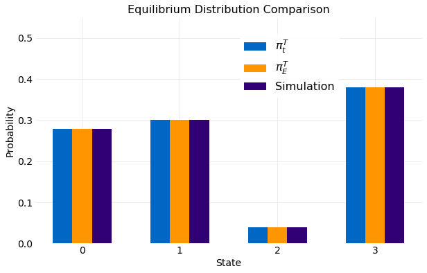The ensemble of samples are collected in the variable chain_samples and plotted below. A comparison is made with the two other calculations performed. The first is $\pi_t$ for $t=100$ shown in equation $(16)$ and the second the solution to equation $(9)$. The different calculations are indistinguishable.

Conclusions

Markov Chain equilibrium for discrete state processes is a general theory of the time evolution of transition probabilities and state distributions. It has been shown that equilibrium is a consequence of assuming the transition matrix and distribution vector are both stochastic. Expressions were derived for the time evolution of any transition matrix and distribution and the equilibrium solutions were then obtained analytically by evaluating the limit $t\to\infty$. A calculation was performed using the obtained equations for the equilibrium solutions and the numpy linear algebra libraries using an example transition matrix. These results were compared to ensemble simulations. The time to relax from an arbitrary state to the equilibrium distributions was shown to occur within $O(10)$ time steps.