Continuous State Markov Chain Equilibrium

A Markov Chain is a sequence of states where transitions between states occur ordered in time with the probability of transition depending only on the previous state. Here the states will be assumed a continuous unbounded set and time a discrete unbounded set. If the set of states is given by, $x\in\mathbb{R}$, the probability that the process will be in state $x$ at time $t$, denoted by $\pi_t (y)$, is referred to as the distribution. Markov Chain equilibrium is defined by $\lim_{t\to\infty}\pi_t (y)\ <\ \infty$, that is, as time advances $\pi_t (y)$ becomes independent of time. Here a solution for this limit is discussed and illustrated with examples.

Model

The Markov Chain is constructed from the set of states $\{x\}$, ordered in time, where $x\in\mathbb{R}$. The process starts at time $t=0$ with state $X_0=x$. At the next step, $t=1$, the process will assume a state $X_1=y$, $y\in\{x\}$, with probability $P(X_1=y|X_0=x)$ since it will depend on the state at $t=0$ by the definition of a Markov Process. At the next time step $t=2$ the process state will be $X_2=z, \text{where}\ z\in\{x\}$ with probability, $P(X_2=z|X_0=x, X_1=y) = P(X_2=z|X_1=y),$ since by definition the probability of state transition depends only upon the state at the previous time step. For an arbitrary time the transition from a state $X_{t}=x$ to a state $X_{t+1}=y$ will occur with probability, $P(X_{t+1}=y|X_t=x)$ that is independent of $t$. The Transition Kernel, defined by,

$p(x,y) = P(X_{t+1}=y|X_t=x),$

plays the same role as the transition matrix plays in the theory of Discrete State Markov Chains. In general $p(x,y)$ cannot always be represented by a probability density function, but here it is assumed that it has a density function representation. This leads to the interpretation that for a known value of $x$ $p(x, y)$ can be interpreted as a conditional probability density for a transition to state $y$ given that the process is in state $x$, namely,

$p(x, y) = f(y|x)$

Consequently, $p(x,y)$ is a family of conditional probability distributions each representing conditioning on a possible state of the chain at time step $t$. Since $p(x, y)$ is a conditional probability density for each value of $x$ it follows that,

$\begin{gathered} \int^{\infty}_{-\infty} p(x, y) dy = 1\ \forall\ x \\ p(x,y)\ \geq 0\ \forall\ x,\ y \end{gathered}\ \ \ \ \ (1).$

The transition kernel for a single step in the Markov Process is defined by $p(x,y)$. The transition kernel across two time steps is computed as follows. Begin by denoting the process state at time $t$ by $X_t=x$, the state at $t+1$ by $X_{t+1}=y$ and the state at $t+2$ by $X_{t+2}=z$. Then the probability of transitioning to a state $X_{t+3}=z$ from $X_{t}=x$ in two steps, $p^2(x, z)$, is given by, $\begin{aligned} f(z|x) &= \int_{-\infty}^{\infty} f(z|x, y)f(y|x) dy \\ &= \int_{-\infty}^{\infty} f(z|y)f(y|x) dy \\ &= \int_{-\infty}^{\infty} p(y,z)p(x,y) dy \\ &= \int_{-\infty}^{\infty} p(x,y)p(y,z) dy \end{aligned}$

where use was made of the Law of Total Probability, in the first step and second step used the Markov Chain property $f(z|x, y)=f(z|y)$. Now, the result obtained for the two step transition kernel is the continuous version of matrix multiplication of the single step transitions probabilities. A operator inspired by matrix multiplication would be helpful. Make the definition, $P^2(x,z) = \int_{-\infty}^{\infty} p(x, y)p(y, z) dy.$

Using this operator, with $X_{t+3}=w$, the three step transition kernel is given by, $\begin{aligned} f(w|x) &= \int_{-\infty}^{\infty} f(w|x,z)f(z|x) dz \\ &= \int_{-\infty}^{\infty} f(w|z) \left[ \int_{-\infty}^{\infty} f(z|y)f(y|x) dy \right] dz \\ &= \int_{-\infty}^{\infty} \int_{-\infty}^{\infty} f(w|z)f(z|y)f(y|x) dy dz \\ &= \int_{-\infty}^{\infty} \int_{-\infty}^{\infty} p(z,w)p(y,z)p(x,y) dy dz \\ &= \int_{-\infty}^{\infty} \int_{-\infty}^{\infty} p(x,y)p(y,z)p(z,w) dy dz \\ &= P^3(x,w), \end{aligned}$

where the second step substitutes the two step transition kernel and the remaining steps perform the decomposition to the single step transition kernel, $p(x,y)$. Use of Mathematical Induction is used to show that the transition kernel between two states in an arbitrary number of steps, $t$, is given by,

$P^t(x,y) = \int_{-\infty}^{\infty}\int_{-\infty}^{\infty}\cdots\int_{-\infty}^{\infty} p(x,z_1)p(z_1,z_2)\ldots p(z_{t-1},y) dz_1 dz_2\ldots dz_{t-1}.$

The distribution of Markov Chain states $\pi (x)$ is defined by,

$\begin{gathered} \int_{-\infty}^{\infty} \pi (x) dx = 1 \\ \pi (x) \geq 0\ \forall\ x \end{gathered}$

To determine the equilibrium distribution, $\pi_E (x)$, the time variability of $\pi_t (x)$ must be determined. Begin by considering an arbitrary distribution at $t=0$, $\pi_0 (x)$. The distribution after the first step will be,

$\pi_1 (y) = \int_{-\infty}^{\infty} p(x, y)\pi_0 (x) dx.$

The distribution after two steps is,

$\begin{aligned} \pi_2 (y) &= \int_{-\infty}^{\infty} p(x, y)\pi_1 (x) dx \\ &= \int_{-\infty}^{\infty} p(x, y)\left[ \int_{-\infty}^{\infty} p(z, x)\pi_0 (z) dz \right] dx \\ &= \int_{-\infty}^{\infty} \int_{-\infty}^{\infty} p(z,x) p(x,y) \pi_0 (z) dx dz \end{aligned}$

The pattern becomes more apparent after the third step,

$\begin{aligned} \pi_3 (y) &= \int_{-\infty}^{\infty} p(x, y)\pi_2 (x) dx \\ &= \int_{-\infty}^{\infty} p(x, y)\left[ \int_{-\infty}^{\infty} \int_{-\infty}^{\infty} p(w,x) p(z,w)\pi_0 (z) dz dw \right] dx \\ &= \int_{-\infty}^{\infty}\int_{-\infty}^{\infty} \int_{-\infty}^{\infty} p(x,y) p(w,x) p(z,w)\pi_0 (z) dz dw dx \\ &= \int_{-\infty}^{\infty}\int_{-\infty}^{\infty} \int_{-\infty}^{\infty} p(z,w) p(w,x) p(x,y) \pi_0 (z) dw dx dz. \end{aligned}$

This looks similar to the previous result obtained for the time dependence of the transition kernel. Making use of the operator $P$ gives,

$\begin{aligned} \pi_1 (y) &= P\pi_0(y) = \int_{-\infty}^{\infty} p(x, y)\pi_0 (x) dx \\ \pi_2 (y) &= P^2\pi_0(y) = \int_{-\infty}^{\infty} \int_{-\infty}^{\infty} p(z,x) p(x,y) \pi_0 (z) dx dz \\ \pi_3 (y) &= P^3\pi_0(y) = \int_{-\infty}^{\infty}\int_{-\infty}^{\infty} \int_{-\infty}^{\infty} p(z,w) p(w,x) p(x,y) \pi_0 (z) dw dx dz. \end{aligned}$

Mathematical Induction can be used to prove the distribution at an arbitrary time $t$ is given by,

$\pi_t (y) = P^t\pi_0(y)\ \ \ \ \ (2)$

Equilibrium Distribution

The equilibrium distribution is defined as the invariant solution to equation $(2)$ for arbitrary $t$, namely,

$\pi_E (y) = P^t\pi_E(y)\ \ \ \ \ (3).$

Consider, $\pi_E (y) = P\pi_E(y)\ \ \ \ \ (4),$

substitution into equation $(3)$ gives,

$\begin{aligned} \pi_E (y) &= P^t\pi_E(y) \\ &= P^{t-1}(P\pi_E)(y) \\ &= P^{t-1}\pi_E(y) \\ &\vdots \\ &= P\pi_E(y) \\ &= \pi_E(y). \end{aligned}$

Thus equation $(4)$ defines the time invariant solution to equation $(3)$.

To go further a particular form for the transition kernel must be specified. Unlike the discrete state model a general solution cannot be obtained since convergence of the limit $t\to\infty$ will depend on the assumed transition kernel. The following section will describe a solution to equation $(4)$ arising from a simple stochastic processes.

Example

To evaluate the equilibrium distribution a form for the transition kernel must be assumed. Here the AR(1) stochastic process is considered. AR(1) is a simple first order autoregressive model providing an example of a continuous state Markov Chain. In following sections its equilibrium distribution is determined and the results of simulations are discussed.

AR(1) is defined by the difference equation,

$X_{t} = \alpha X_{t-1} + \varepsilon_{t}\ \ \ \ \ (5),$

where $t=0,\ 1,\ 2,\ldots$ and the $\varepsilon_{t}$ are identically distributed independent $\textbf{Normal}$ random variables with zero mean and variance, $\sigma^2$. The $t$ subscript on $\varepsilon$ indicates that it is generated at time step $t$. The transition kernel for AR(1) can be derived from equation $(5)$ by using, $\varepsilon_{t} \sim \textbf{Normal}(0,\ \sigma^2)$ and letting $x=x_{t-1}$ and $y=x_{t}$ so that $\varepsilon_{t} = y - \alpha x$. The result is,

$p(x,y) = \frac{1}{\sqrt{2\pi\sigma^2}} e^{-(y-\alpha x)^2/2\sigma^2}\ \ \ \ \ \ (6)$

Now, consider a few steps,

$\begin{aligned} X_1 &= \alpha X_0 + \varepsilon_1 \\ X_2 &= \alpha X_1 + \varepsilon_2 \\ X_3 &= \alpha X_2 + \varepsilon_3, \end{aligned}$

substituting the first equation into the second equation and that result into the third equation gives,

$X_3 = \alpha^3 X_0 + \alpha^2\varepsilon_1 + \alpha\varepsilon_2 + \varepsilon_3$

If this process is continued for $t$ steps the following result is obtained,

$X_t = \alpha^t X_0 + \sum_{i=1}^{t} \alpha^{t-i} \varepsilon_{i}\ \ \ \ \ (7).$

Equilibrium Solution

In this section equation $(7)$ is used to evaluate the the mean and variance of the AR(1) process in the equilibrium limit $t\to\infty$. The mean and variance obtained are then used to construct $\pi_E(x)$ that is shown to be a solution to equation $(4)$.

The equilibrium mean is given by,

$\mu_{E} = \lim_{t\to\infty} E(X_t).$

From equation $(7)$ it is seen that,

$\begin{aligned} E(X_t) &= E\left[ \alpha^t X_0 + \sum_{i=1}^{t} \alpha^{t-i} \varepsilon_{i} \right] \\ &= \alpha^t x_0 + \sum_{i=1}^t E(\varepsilon_i) \\ &= \alpha^t x_0, \end{aligned}$

where the last step follows from $E(\varepsilon_i)=0$. Now,

$\begin{aligned} \mu_E &= \lim_{t\to\infty} E(X_t) \\ &= \lim_{t\to\infty} \alpha^t X_0, \end{aligned}$

this limit exists for $\mid\alpha\mid\ \leq\ 1$,

$\mu_E = \begin{cases} X_0 & \mid\alpha\mid=1 \\ 0 & \mid\alpha\mid\ \leq\ 1 \end{cases}\ \ \ \ \ (8).$

The equilibrium variance is given by,

$\sigma^2_E = \lim_{t\to\infty} E(X^2_t) - \left[E(X_t)\right]^2.$

To evaluate this expression and equation for $X^2_t$ is needed. From equation $(7)$ it follows that,

$\begin{aligned} X_t^2 &= \left[ \alpha^t X_0 + \sum_{i=1}^{t} \alpha^{t-i} \varepsilon_i \right]^2 \\ &= \alpha^{2t}X_0^2 + 2\alpha^t X_0\sum_{i=1}^t \alpha^{t-1} \varepsilon_i + \sum_{i=1}^t \sum_{j=1}^t \alpha^{t-i}\alpha^{t-j}\varepsilon_i \varepsilon_j. \end{aligned}$

It follows that,

$\begin{aligned} E(X_t^2) &= E\left[\alpha^{2t}X_0^2 + 2\alpha^t X_0\sum_{i=1}^t \alpha^{t-1} \varepsilon_i + \sum_{i=1}^t \sum_{j=1}^t \alpha^{t-i}\alpha^{t-j}\varepsilon_i \varepsilon_j \right] \\ &= \alpha^{2t} X_0^2 + 2\alpha^t X_0\sum_{i=1}^t \alpha^{t-1} E(\varepsilon_i) + \sum_{i=1}^t \sum_{j=1}^t \alpha^{t-i}\alpha^{t-j}E(\varepsilon_i \varepsilon_j) \\ &= \alpha^{2t} X_0^2 + \sum_{i=1}^t \sum_{j=1}^t \alpha^{t-i}\alpha^{t-j}E(\varepsilon_i \varepsilon_j), \end{aligned}$

where the last step follows from $E(\varepsilon_i)=0$. Since the $\varepsilon_t$ are independent,

$E(\varepsilon_i \varepsilon_j) = \sigma^2 \delta_{ij},$

where $\delta_{ij}$ is the Kronecker Delta, $\delta_{ij} = \begin{cases} 0 & i \neq j \\ 1 & i=j \end{cases}.$

Using these results gives,

$\begin{aligned} E(X_t^2) &= \alpha^{2t} X_0^2 + \sigma^2\sum_{i=1}^t \sum_{j=1}^t \alpha^{2t-i-j}\delta_{ij} \\ &= \alpha^{2t} X_0^2 + \sigma^2\sum_{i=1}^t \alpha^{2(t-i)} \\ &= \alpha^{2t} X_0^2 + \sigma^2\sum_{i=1}^t \left(\alpha^2\right)^{t-i} \\ &= \alpha^{2t} X_0^2 + \frac{\sigma^2\left[1 - (\alpha^2)^{t-1}\right]}{1 - \alpha^2}, \end{aligned}$

The last step follows from summation of a geometric series,

$\begin{aligned} \sum_{i=1}^{t} (\alpha^2)^{t-1} &= \sum_{k=0}^{t-1}(\alpha^2)^k \\ &= \frac{1-(\alpha^2)^{t-1}}{1-\alpha^2}. \end{aligned}$

In the limit $t\to\infty$ $E(X_t^2)$ only converges for $\mid\alpha\mid\ <\ 1$. If $\alpha=1$ the denominator of the second term in of $E(X_t^2)$ is $0$ $E(X_t^2)$ is undefined. $\sigma^2_E$ is evaluated assuming $\mid\alpha\mid\ <\ 1$ if this is the case $(8)$ gives $\mu_E=0$, so,

$\begin{aligned} \sigma^2_E &= \lim_{t\to\infty} E(X_t^2) - \left(\mu_E\right)^2 \\ &= \lim_{t\to\infty} \alpha^{2t}X_0^2 + \frac{\sigma^2\left[1 - (\alpha^2)^{t-1}\right]}{1 - \alpha^2} \\ &= \frac{\sigma^2}{1 - \alpha^2}. \end{aligned}\ \ \ \ \ (9)$

The equilibrium distribution, $\pi_E$, is found by substituting the results from equation $(8)$ and $(9)$ into a $\textbf{Normal}(\mu_E,\ \sigma^2_E)$ distribution to obtain,

$\pi_E(y) = \frac{1}{\sqrt{2\pi\sigma_E^2}}e^{-y^2/2\sigma_E^2}\ \ \ \ \ (10)$

It can be shown that equation $(10)$ is the equilibrium distribution by verifying that it is a solution to equation $(4)$. Inserting equations $(6)$ and $(10)$ into equation $(4)$ yields,

$\begin{aligned} P\pi_E(y) &= \int_{-\infty}^{\infty} p(x, y) \pi_E(x) dx \\ &= \int_{-\infty}^{\infty} \left[\frac{1}{\sqrt{2\pi\sigma^2}} e^{(y-\alpha x)^2/2\sigma^2}\right]\left[\frac{1}{\sqrt{2\pi\sigma_E^2}}e^{-y^2/2\sigma_E^2}\right] dx \\ &= \frac{1}{\sqrt{2\pi\sigma^2}}\frac{1}{\sqrt{2\pi\sigma_E^2}} \int_{-\infty}^{\infty} e^{-\frac{1}{2}\left[(y-\alpha x)^2/\sigma^2+x^2/\sigma_E^2 \right]} dx \\ &= \frac{1}{\sqrt{2\pi\sigma^2}}\frac{1}{\sqrt{2\pi\sigma_E^2}} \int_{-\infty}^{\infty} e^{-\frac{1}{2}\left[y^2/\sigma_E^2+(x-\alpha y)^2/\sigma^2 \right]} dx \\ &= \frac{1}{\sqrt{2\pi\sigma_E^2}} e^{-y^2/2\sigma_E^2}\frac{1}{\sqrt{2\pi\sigma^2}}\int_{-\infty}^{\infty} e^{-(x-\alpha y)^2/2\sigma^2} dx \\ &= \frac{1}{\sqrt{2\pi\sigma_E^2}} e^{-y^2/2\sigma_E^2} \\ &= \pi_E(y) \end{aligned}$

Simulation

An AR(1) simulator can be implemented using either the difference equation definition, equation $(5)$ or the transition kernel, equation $(6)$. The result produced by either are statistically identical, An example implementation in Python using equation $(5)$ is shown below.

def ar_1_difference_series(α, σ, x0, nsample=100):
    samples = numpy.zeros(nsample)
    ε = numpy.random.normal(0.0, σ, nsample)
    samples[0] = x0
    for i in range(1, nsample):
        samples[i] = α * samples[i-1] + ε[i]
    return samples

The function ar_1_difference_series(α, σ, x0, nsamples) takes four arguments: α and σ, the initial value of $x$, x0 and the number of desired samples nsample. It begins by allocating storage for the sample output followed by generation of nsample values of $\varepsilon_\sim \textbf{Normal}(0,\ \sigma^2)$ with the requested standard deviation, $\sigma$. The samples are then created using the AR(1 ) difference equation, equation $(5)$. A second implementation using the transition kernel, equation $(6)$ is shown below.

def ar1_kernel_series(α, σ, x0, nsample=100):
    samples = numpy.zeros(nsample)
    samples[0] = x0
    for i in range(1, nsample):
        samples[i] = numpy.random.normal(α * samples[i-1], σ)
    return samples

The function ar1_kernel_series(α, σ, x0, nsamples) also takes four arguments: α and σ from equation $(6)$, the initial value of $x$, x0 and the number of desired samples, nsample. It begins by allocating storage for the sample output and then generates samples using the transition kernel with distribution $\textbf{Normal}(α * samples[i-1],\ \sigma^2)$.

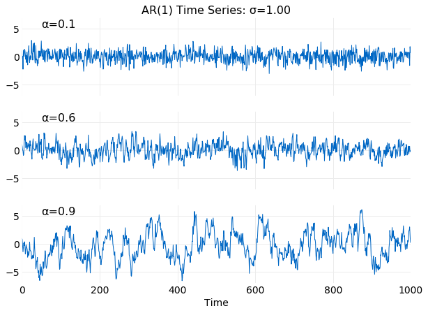
The plots below show examples of time series generated using ar_1_difference_series with $\sigma=1$ and values of $\alpha$ satisfying $\alpha\ <\ 1$. It is seen that for smaller $\alpha$ values of the series more frequently change direction and have smaller variance. This is expected from equation $(9)$, where $\sigma_E=1/1-\alpha^2$.

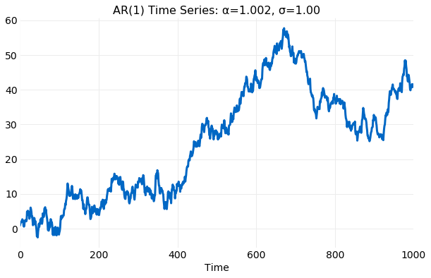
If $\alpha$ is just slightly larger than $1$ the time series can increase rapidly as illustrated in the plot below.

For $\alpha\ <\ 1$ $\sigma_E$ is bounded and the generated samples are constrained about the equilibrium mean value, $\mu_E=0$, but for $\alpha\ \geq\ 1$ $\sigma_E$ is unbounded and the samples very quickly develop very large deviations from $\mu_E$.

Convergence to Equilibrium

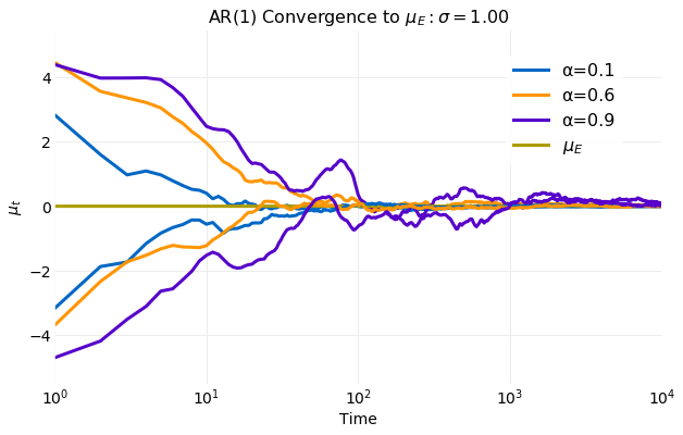
For sufficiently large times samples generated by the AR(1) process will approach the equilibrium values for $\alpha\ <\ 1$. In the plots following the cumulative values of both the mean and standard deviation computed from simulations, using ar_1_difference_series with $\sigma=1$, are compared with the equilibrium vales $\mu_E$ and $\sigma_E$ from equations $(8)$ and $(9)$ respectively. The first plot illustrates the convergence $\mu$ to $\mu_E$ for six different simulations with varying initial states, $X_0$, and $\alpha$. The rate of convergence is seen to decrease as $\alpha$ increases. For smaller $\alpha$ the simulation $\mu$ is close to $\mu_E$ within $10^2$ samples and indistinguishable from $\mu_E$ by $10^3$. For larger values of $\alpha$ the convergence is mush slower. After $10^5$ samples there are still noticeable oscillations of the sampled $\mu$ about $\mu_E$.

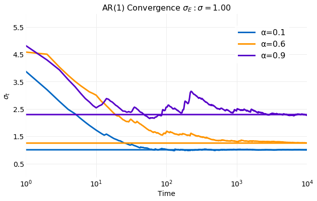
Since $\sigma_E$ varies with $\alpha$ for clarity only simulations with varying $\alpha$ are shown. The rate of convergence $\sigma$ to $\sigma_E$ is slightly slower than the rate seem for $\mu$. For smaller $\alpha$ simulation $\sigma$ computations are indistinguishable form $\sigma_E$ by $10^3$ samples. For larger $\alpha$ after $10^4$ sample deviations about the $\sigma_E$ are still visible.

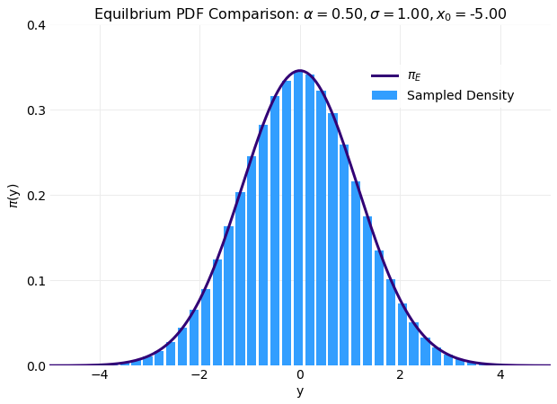
The plot below favorably compares the histogram produced from results of a simulation of $10^6$ samples and the equilibrium distribution, $\pi_E(y)$, from equation $(10)$.

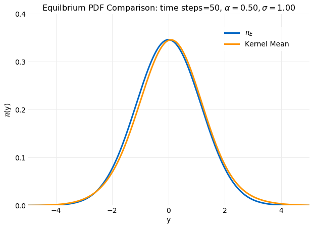
A more efficient method of estimating $\pi_E(y)$ is obtained from equation $(4)$ by noting that for sufficiently large number of samples equation $(4)$ can be approximated by the expectation of the transition kernel, namely,

$\begin{aligned} \pi_E(y) &= P\pi_E(y) \\ &= \int_{-\infty}^{\infty} p(x, y) \pi_E(x) dx \\ &\approx \frac{1}{N} \sum_{i=0}^{N-1} p(x_i, y). \end{aligned}\ \ \ \ \ (11)$

A Python implementation of the solution to equation $(11)$ for the average transition kernel is listed below where two functions are defined.

def ar_1_kernel(α, σ, x, y):
    p = numpy.zeros(len(y))
    for i in range(0, len(y)):
        ε  = ((y[i] -  α * x)**2) / (2.0 * σ**2)
        p[i] = numpy.exp(-ε) / numpy.sqrt(2 * numpy.pi * σ**2)
    return p

def ar_1_equilibrium_distributions(α, σ, x0, y, nsample=100):
    py = [ar_1_kernel(α, σ, x, y) for x in ar_1_difference_series(α, σ, x0, nsample)]
    pavg = [py[0]]
    for i in range(1, len(py)):
        pavg.append((py[i] + i * pavg[i-1]) / (i + 1))
    return pavg

The first function ar_1_kernel(α, σ, x, y) computes the transition kernel for a range of values and takes four arguments as input: α and σ from equation $(5)$ and the value of x and an array of y values where the transition kernel is evaluated. The second function ar_1_equilibrium_distributions(α, σ, x0, y, nsample) has five arguments as input:
α and σ, the initial value of $x$, x0, the array of y values used to evaluate the transition kernel and the number of desired samples nsample. ar_1_equilibrium_distributions begins by calling ar_1_difference_series to generate nsample samples of x. These values and the needed inputs are then passed to ar_1_kernel providing nsample evaluations of the transition kernel. The cumulative average of the transition kernel is then evaluated and returned.

In practice this method gives reasonable results for as few as $10^2$ samples. This is illustrated in the following plot where the transition kernel mean value computed with just $50$ samples using ar_1_equilibrium_distributions is compared $\pi_E(y)$ from equation $(10)$.

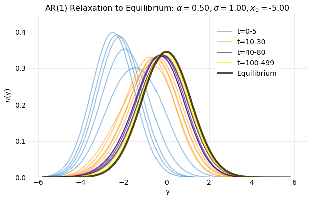
The following plot shows intermediate values the calculation in the range of $1$ to $50$ samples. This illustrates the changes in the estimated equilibrium distribution as the calculation progresses. By $500$ samples a distribution near the equilibrium distribution is obtained.

Conclusions

Markov Chain equilibrium for continuous state processes provides a general theory of the time evolution of stochastic kernels and distributions. Unlike the case for the discrete state model general solutions cannot be obtained since evaluation of the obtained equations depends of the form of the stochastic kernel. Kernels will exist which do not have equilibrium solutions. A continuous state process that has an equilibrium distribution that can be analytically evaluated is AR(1). The stochastic kernel for AR(1) is derived from its difference equation representation and the first and second moments are evaluated in the equilibrium limit, ${t\to\infty}$. It is shown that finite values exists only for values of the AR(1) parameter that satisfy $\mid\alpha\mid\ < \ 1$. A distribution is then constructed using these moments and shown to be the equilibrium distribution. Simulations are performed using the difference equation representation of the process and compared with the equilibrium calculations. The rate of convergence of simulations to the equilibrium is shown to depend on $\alpha$. For values not near $1$ convergence of the mean occurs with $O(10^3)$ time steps and convergence of the standard deviation with $O(10^4)$ time steps. For values of $\alpha$ closer to $1$ convergence has not occurred by $10^4$ time steps.