Discrete Cross Correlation Theorem

The Cross Correlation Theorem is similar to the more widely known Convolution Theorem. The cross correlation of two discrete finite time series $\{f_0,\ f_1,\ f_2,\ldots\,\ f_{N-1}\}$ and $\{g_0,\ g_1,\ g_2,\ldots\,\ g_{N-1}\}$ is defined by,

$\psi_t = \sum_{n=0}^{N-1} f_{n} g_{n+t}\ \ \ \ \ (1),$

where $t$ is called the time lag. Cross correlation provides a measure of the similitude of two time series when shifted by the time lag. A direct calculation of the cross correlation using the equation above requires $O(N^2)$ operations. The Cross Correlation Theorem provides a method for calculating cross correlation in $O(NlogN)$ operations by use of the Fast Fourier Transform. Here the theoretical background required to understand cross correlation calculations using the Cross Correlation Theorem is discussed. Example calculations are performed and different implementations using the FFT libraries in numpy compared. The important special case of the cross correlation called Autocorrelation is addressed in the final section.

Cross Correlation

Cross Correlation can be understood by considering the Covariance of two random variables, $X$ and $Y$. Covariance is the Expectation of the product of the deviations of the random variables from their respective means,

$\begin{aligned} Cov(X,Y) &= E\left[(X-E[X])(Y-E[Y])\right] \\ &= E[XY] - E[X]E[Y]. \end{aligned}\ \ \ \ \ (2)$

Note that $Cov(X,Y)=Cov(Y,X)$ and if $X$ and $Y$ are Independent Random Variables $E[XY]=E[X]E[Y]\ \implies\ Cov(X,Y)=0$. If $X=Y$ the Covariance reduces to the Variance,

$\begin{aligned} Var(X) &= E\left[(X-E[X])^2\right] \\ &= E[X^2] - \left(E[X]\right)^2. \end{aligned}$

These two results are combined in the definition of the Correlation Coefficient,

$\rho_{XY} = \frac{Cov(X,Y)}{\sqrt{Var(X)Var(Y)}}.$

The correlation coefficient has a geometric interpretation leading to the conclusion that $-1\ \leq \rho_{XY}\ \leq 1$. At the extreme values $X$ and $Y$ are either the same or differ by a multiple of $-1$. At the midpoint value, $\rho_{XY}=0$, $X$ and $Y$ are independent random variables. If follows that $\rho_{XY}$ provides a measure of possible dependence or similarity of two random variables.

Consider the first term in equation $(2)$ when a time series of samples of $X$ and $Y$ of equal length are available,

$\begin{aligned} E[XY]& \approx \frac{1}{N^2}\sum_{n=0}^{N-1}x_n y_n \\ &\propto\ \psi_{0}, \end{aligned}$

if $N$ is sufficiently large. Generalizing this result to arbitrary time shifts leads to equation $(1)$.

An important special case of the cross correlation is the autocorrelation which is defined a the cross correlation of a time series with itself,

$r_t = \sum_{n=0}^{N-1} x_{n} x_{n+t}\ \ \ \ \ (3).$

Building on the interpretation of cross correlation the autocorrelation is viewed as a measure of dependence or similarity of the past and future of a time series. For a time lag of $t=0$,

$r_0\ \propto\ E\left[X^2\right].$

Discrete Fourier Transform

This section will discuss properties of the Discrete Fourier Transform that are used in following sections. The Discrete Fourier Transform for a discrete periodic time series of length $N$, $\{f_0,\ f_1,\ f_2,\ldots,\ f_{N-1}\}$, is defined by,

$\begin{gathered} f_{n} = \frac{1}{N}\sum_{k=0}^{N-1}F_{k}e^{2\pi i (k/N)n} \\ F_{k} = \sum_{n=0}^{N-1}f_{n}e^{-2\pi i (n/N)k}, \end{gathered}\ \ \ \ \ (4)$

where the expression for $f_{n}$ is referred to the inverse transform and the one for $F_{k}$ the forward transform.

Linearity

Both the forward and inverse transforms are Linear Operators. An operator, $\mathfrak{F}$, is linear if the operation on a sum is equal the sum of the operations,

$\mathfrak{F}(a+b) = \mathfrak{F}(a)+\mathfrak{F}(b)\ \ \ \ \ (5)$

To show this for the forward transform consider $h_{n}=f_{n}+g_{n}$, then,

$\begin{aligned} H_{k} &= \sum_{n=0}^{N-1}h_{n}e^{-2\pi i (n/N)k} \\ &= \sum_{n=0}^{N-1}\left(f_{n}+g_{n}\right)e^{-2\pi i (n/N)k} \\ &= \sum_{n=0}^{N-1}f_{n} e^{-2\pi i (n/N)k} + \sum_{n=0}^{N-1} g_{n}e^{-2\pi i (n/N)k} \\ &= F_{k} + G_{k}. \end{aligned}$

Similarly it can be shown that the inverse transform is linear.

Periodicity

Periodicity of the forward transform implies that, $F_{k+mN}=F_{k}\ \ \ \ \ (6),$ where $m=\{\ldots,-2,\ -1,\ 0,\ 1,\ 2,\ldots\}$. To show that this is true first consider the case $m=1$,

$\begin{aligned} F_{k+N} &= \sum_{n=0}^{N} f_{n}e^{-2\pi i (n/N)(k+N)} \\ &= \sum_{n=0}^{N} f_{n} e^{-2\pi i(n/N)k}e^{-2\pi i n} \\ &= \sum_{n=0}^{N} f_{n} e^{-2\pi i(n/N)k} \\ &= F_{k}, \end{aligned}$

where the second step follows from, $e^{2\pi i n} = 1,\ \forall\ n$.

For an arbitrary value of $m$, $\begin{aligned} F_{k+mN} &= \sum_{n=0}^{N} f_{n}e^{-2\pi i (n/N)(k+mN)} \\ &= \sum_{n=0}^{N} f_{n} e^{-2\pi i(n/N)k}e^{-2\pi i nm} \\ &= \sum_{n=0}^{N} f_{n} e^{-2\pi i(n/N)k} \\ &= F_{k}, \end{aligned}$

since, $e^{2\pi i mn} = 1,\ \forall\ m,\ n$.

Consequence of Real $f_{n}$

If $f_{n}$ is real then $f_{n}=f_{n}^{\ast}$, where $\ast$ denotes the Complex Conjugate. It follows that,

$\begin{aligned} f_{n} &= f_{n}^{\ast} \\ &= \left\{ \frac{1}{N}\sum_{k=0}^{N-1}F_{k}e^{2\pi i (k/N)n} \right\}^{\ast} \\ &= \frac{1}{N}\sum_{k=0}^{N-1}F_{k}^{\ast}e^{-2\pi i (k/N)n} \end{aligned}\ \ \ \ \ (7)$

Another interesting and related result is,

$F_{-k} = F_{k}^{\ast}\ \ \ \ \ (8).$

which follows from,

$\begin{aligned} F_{-k} &= \sum_{n=0}^{N-1} f_{n}e^{2\pi i (n/N)k} \\ &= \sum_{n=0}^{N-1} f_{n}^{\ast}e^{2\pi i (n/N)k} \\ &= \left\{ \sum_{n=0}^{N-1} f_{n}e^{-2\pi i (n/N)k}\right\}^{\ast} \\ &=F_{k}^{\ast}. \end{aligned}$

Orthogonality of Fourier Basis

The Discrete Fourier Basis is the collection of functions,

$\left\{e^{2\pi i(k/N)n}\right\},$

where $n = 0,\ 1,\ 2,\ldots,N-1$. It forms an Orthogonal Basis since,

$\frac{1}{N} \sum_{n=0}^{N-1} e^{2\pi \left[ (m-k)/N\right] n}\ =\ \delta_{mk} = \begin{cases} 1 & \text{if}\ m\ =\ k \\ 0 & \text{if}\ m\ \ne\ k \end{cases}\ \ \ \ \ (9),$

where $\delta_{mk}$ is the Kronecker Delta. This result can be proven for $m\ \ne\ k$ by noting that the sum in equation $(9)$ is a Geometric Series,

$\frac{1}{N} \sum_{n=0}^{N-1} e^{2\pi i \left[(m-k)/N \right] n} = \frac{1}{N} \frac{1-e^{2\pi i (m-k)}}{1-e^{2\pi i (m-k)/N}}.$

Since $2\pi i(m-k)$ is always a multiple of $2\pi$ it follows that the numerator is zero,

$1-e^{2\pi i (m-k)} = 1-1 = 0.$

The denominator is zero only if $m-k=lN$ where $l$ is an integer. This cannot happen since $-(N-1)\ \leq m-k\ \leq N-1$, so,

$\sum_{n=0}^{N-1} e^{2\pi \left[ (m-k)/N\right] n}\ =\ 0$

If $m=k$ then,

$\sum_{n=0}^{N-1} e^{2\pi i \left[(m-k)/N \right] n} = \sum_{n=0}^{N-1} 1 = N,$

this proves that equation $(9)$.

The Cross Correlation Theorem

The Cross Correlation Theorem is a relationship between the Fourier Transform of the cross correlation, $\psi_{t}$ defined by equation $(1)$ and the Fourier Transforms of the two time series used in the cross correlation calculation,

$\Psi_{k} = F_{k}^{\ast}G_{k}\ \ \ \ \ (10),$

where,

$\begin{aligned} \Psi_{k} &= \sum_{n=0}^{N-1}\psi_{n}e^{-2\pi i (n/N)k} \\ F_{k}^{\ast} &= \sum_{n=0}^{N-1}f_{n}^{\ast}e^{2\pi i (n/N)k} \\ G_{k} &= \sum_{n=0}^{N-1}g_{n}e^{-2\pi i (n/N)k}. \end{aligned}$

To derive equation $(10)$ consider the Inverse Fourier Transform of the time series $f_{n}$ and $g_{n+t}$,

$\begin{gathered} f_{n} = \frac{1}{N}\sum_{k=0}^{N-1}F_{k}^{\ast}e^{-2\pi i (k/N)n} \\ g_{n+t} = \frac{1}{N}\sum_{k=0}^{N-1}G_{k}e^{2\pi i (k/N)(n+t)}, \end{gathered}$

Substituting these expressions into equation $(1)$ gives,

$\begin{aligned} \psi_t &= \sum_{n=0}^{N-1} f_{n} g_{n+t} \\ &= \sum_{n=0}^{N-1} \left\{ \frac{1}{N}\sum_{k=0}^{N-1}F_{k}^{\ast}e^{-2\pi i (k/N)n} \right\} \left\{ \frac{1}{N}\sum_{m=0}^{N-1}G_{m}e^{2\pi i (m/N)(n+t)} \right\} \\ &= \frac{1}{N}\sum_{k=0}^{N-1}\sum_{m=0}^{N-1} F_{k}^{\ast}G_{m} e^{2\pi i (t/N)m} \frac{1}{N} \sum_{n=0}^{N-1} e^{2\pi i \left[(m-k)/N \right] n} \\ &= \frac{1}{N}\sum_{k=0}^{N-1}\sum_{m=0}^{N-1} F_{k}^{\ast}G_{m} e^{2\pi i (t/N)m} \delta_{mk} \\ &= \frac{1}{N}\sum_{k=0}^{N-1} F_{k}^{\ast}G_{k} e^{2\pi i (t/N)k}, \end{aligned}$

where the second step follows from equation $(9)$. Equation $(10)$ follows by taking the Fourier Transform of the previous result,

$\begin{aligned} \Psi_{k} &= \sum_{t=0}^{N-1}\psi_{t}e^{-2\pi i (t/N)k} \\ &= \sum_{t=0}^{N-1} \left\{ \frac{1}{N}\sum_{k=0}^{N-1} F_{k}^{\ast}G_{k} e^{2\pi i (t/N)m} \right\}e^{-2\pi i (t/N)k} \\ &= \sum_{m=0}^{N-1} F_{m}^{\ast}G_{m} \frac{1}{N} \sum_{t=0}^{N-1} e^{2\pi i \left[(m-k)/N)\right]t} \\ &= \sum_{m=0}^{N-1} F_{m}^{\ast}G_{m} \delta_{mk} \\ &= F_{k}^{\ast}G_{k}, \end{aligned}$

proving the Cross Correlation Theorem defined by equation $(10)$.

Discrete Fourier Transform Example

This section will work through an example calculation of a discrete Fourier Transform that can be worked out by hand. The manual calculations will be compared with calculations performed using the FFT library from numpy.

The Discrete Fourier Transform of a time series, represented by the column vector $f$, into a column vector of Fourier coefficients, $\overline{f}$, can be represented by the linear equation,

$\overline{f} = Tf,$

where $T$ is the transform matrix computed from the Fourier basis functions. Each element of the matrix is the value of the basis function used in the calculation. It is assumed that the time series contains only $4$ points so that $T$ will be a $4\times 4$ matrix. The transform matrix only depends on the number of elements in the time series vector and is given by,

$T= \begin{pmatrix} 1 & 1 & 1 & 1 \\ 1 & e^{-i\pi/2} & e^{-i\pi} & e^{-i3\pi/2} \\ 1 & e^{-i\pi} & e^{-i2\pi} & e^{-i3\pi} \\ 1 & e^{-i3\pi/2} & e^{-i3\pi} & e^{-i9\pi/2} \end{pmatrix} = \begin{pmatrix} 1 & 1 & 1 & 1 \\ 1 & -i & -1 & i \\ 1 & -1 & 1 & -1 \\ 1 & i & -1 & -i \end{pmatrix} \ \ \ \ \ (11)$

Assume an example time series of,

$f = \begin{pmatrix} 8 \\ 4 \\ 8 \\ 0 \end{pmatrix}.$

It follows that,

$\begin{aligned} \begin{pmatrix} \overline{f_1} \\ \overline{f_2} \\ \overline{f_3} \\ \overline{f_4} \end{pmatrix} &= \begin{pmatrix} 1 & 1 & 1 & 1 \\ 1 & -i & -1 & i \\ 1 & -1 & 1 & -1 \\ 1 & i & -1 & -i \end{pmatrix} \begin{pmatrix} 8 \\ 4 \\ 8 \\ 0 \end{pmatrix} \\ &= \begin{pmatrix} 20 \\ -4i \\ 12 \\ 4i \end{pmatrix} \end{aligned}\ \ \ \ \ (12)$

The Python code listing below uses the FFT implementation from numpy to confirm the calculation of equation $(12)$. It first defines the time series example data $f$. The Fourier Transform is then used to compute $\overline{f}$.

In [1]: import numpy
In [2]: f = numpy.array([8, 4, 8, 0])
In [3]: numpy.fft.fft(f)
Out[3]: array([20.+0.j,  0.-4.j, 12.+0.j,  0.+4.j])

Cross Correlation Theorem Example

This section will work through an example calculation of cross correlation using the Cross Correlation Theorem with the goal of verifying an implementation of the algorithm in Python. Here use will be made of the time series vector $f$ and the transform matrix $T$ discussed in the previous section. An additional time series vector also needs to be considered, let,

$g = \begin{pmatrix} 6 \\ 3 \\ 9 \\ 3 \end{pmatrix}.$

First, consider a direct calculation of the cross correlation, $\psi_t = \sum_{n=0}^{N-1} f_{n} g_{n+t}$. The following python function cross_correlate_sum(x, y) implements the required summation.

In [1]: import numpy
In [2]: def cross_correlate_sum(x, y):
   ...:     n = len(x)
   ...:     correlation = numpy.zeros(len(x))
   ...:     for t in range(n):
   ...:         for k in range(0, n - t):
   ...:             correlation[t] += x[k] * y[k + t]
   ...:     return correlation
   ...:

In [3]: f = numpy.array([8, 4, 8, 0])
In [4]: g = numpy.array([6, 3, 9, 3])
In [5]: cross_correlate_sum(f, g)
Out[5]: array([132.,  84.,  84.,  24.])

cross_correlate_sum(x, y) takes two vectors, x and y, as arguments. It assumes that x and y are equal length and after allocating storage for the result performs the double summation required to compute the cross correlation for all possible time lags, returning the result. It is also seen that $O(N^2)$ operations are required to perform the calculation, where $N$ is the length of the input vectors.

Verification of following results requires a manual calculation. A method of organizing the calculation to facilitate
this is shown in table below. The table rows are constructed from the elements of $f_{n}$ and the time lagged elements of $g_{n+t}$ for each value $t$. The column is indexed by the element number $n$. The time lag shift performed on the vector $g_{n+t}$ results in the translation of the components to the left that increases for each row as the time lag increases. Since the number of elements in $f$ and $g$ is finite the time lag shift will lead to some elements not participating in $\psi_{t}$ for some time lag values. If there is no element in the table at a position the value of $f$ or $g$ at that position is assumed to be $0$.

$n$				0	1	2	3
$f_{n}$				8	4	8	0
$g_{n}$				6	3	9	3
$g_{n+1}$			6	3	9	3
$g_{n+2}$		6	3	9	3
$g_{n+3}$	6	3	9	3

The cross correlation, $\psi_t$, for a value of the time lag, $t$, is computed for each $n$ by multiplication of $f_{n}$ and $g_{n+t}$ and summing the results. The outcome of this calculation is shown as the column vector $\psi$ below where each row corresponds to a different time lag value.

$\psi = \begin{pmatrix} 8\cdot 6 + 4\cdot 3 + 8\cdot 9 + 0\cdot 3 \\ 8\cdot 3 + 4\cdot 9 + 8\cdot 3 \\ 8\cdot 9 + 4\cdot 3 \\ 8\cdot 3 \end{pmatrix} = \begin{pmatrix} 132 \\ 84 \\ 84 \\ 24 \end{pmatrix}\ \ \ \ \ \ (13)$

The result is the same as determined by cross_correlate_sum(x,y).

Now that an expectation of a result is established it can be compared with the a calculation using using the Cross Correlation Theorem from equation $(10)$ where $f$ and $g$ are represented by Discrete Fourier Series. It was previously shown that the Fourier representation is periodic, see equation $(6)$. It follows that the time lag shifts of $g_{n+t}$ will by cyclic as shown in the calculation table below.

$n$	0	1	2	3
$f_{n}$	8	4	8	0
$g_{n}$	6	3	9	3
$g_{n+1}$	3	9	3	6
$g_{n+2}$	9	3	6	3
$g_{n+3}$	3	6	3	9

Performing the calculation following the steps previously described has the following outcome,

$\psi = \begin{pmatrix} 8\cdot 6 + 4\cdot 3 + 8\cdot 9 + 0\cdot 3 \\ 8\cdot 3 + 4\cdot 9 + 8\cdot 3 + 0\cdot 6 \\ 8\cdot 9 + 4\cdot 3 + 8\cdot 6 + 0\cdot 3 \\ 8\cdot 3 + 4\cdot 6 + 8\cdot 3 + 0\cdot 9 \end{pmatrix} = \begin{pmatrix} 132 \\ 84 \\ 132 \\ 72 \end{pmatrix}.$

This is different from what was obtained from a direct evaluation of the cross correlation sum. Even though the result is different the calculation could be correct since periodicity of $f$ and $g$ was not assumed when the sum was evaluated. Below a calculation using the Cross Correlation Theorem implemented in Python is shown.

In [1]: import numpy
In [2]: f = numpy.array([8, 4, 8, 0])
In [3]: g = numpy.array([6, 3, 9, 3])
In [4]: f_bar = numpy.fft.fft(f)
In [5]: g_bar = numpy.fft.fft(g)
In [6]: numpy.fft.ifft(f_bar * g_bar)
Out[6]: array([132.+0.j,  72.+0.j, 132.+0.j,  84.+0.j])

In the calculation $f$ and $g$ are defined and their Fourier Transforms are computed. The Cross Correlation Theorem is then used to compute the Fourier Transform of the cross correlation, which is then inverted. The result obtained is the same as obtained in the manual calculation verifying the results. Since the calculations seem to be correct the problem must be that periodicity of the Fourier representations $f$ and $g$ was not handled properly. This analysis artifact is called aliasing. The following example attempts to correct for this problem.

The cross correlation calculation table for periodic $f$ and $g$ can be made to resemble the table for the nonperiodic case by padding the end of the vectors with $N-1$ zeros, where $N$ is the vector length, creating a new periodic vector of length $2N-1$. This new construction is shown below.

$n$				0	1	2	3	4	5	6
$f_{n}$				8	4	8	0
$g_{n}$				6	3	9	3	0	0	0
$g_{n+1}$			6	3	9	3	0	0	0	6
$g_{n+2}$		6	3	9	3	0	0	0	6	3
$g_{n+3}$	6	3	9	3	0	0	0	6	3	9
$g_{n+4}$	3	9	3	0	0	0	6	3	9	3
$g_{n+5}$	9	3	0	0	0	6	3	9	3	0
$g_{n+6}$	3	0	0	0	6	3	9	3	0	0

It follows that,

$\psi = \begin{pmatrix} 8\cdot 6 + 4\cdot 3 + 8\cdot 9 + 3\cdot 0 \\ 8\cdot 3 + 4\cdot 9 + 8\cdot 3 + 0\cdot 0 \\ 8\cdot 9 + 4\cdot 3 + 8\cdot 0 + 0\cdot 0 \\ 8\cdot 3 + 4\cdot 0 + 8\cdot 0 + 0\cdot 0 \\ 8\cdot 0 + 4\cdot 0 + 8\cdot 0 + 0\cdot 3 \\ 8\cdot 0 + 4\cdot 0 + 8\cdot 6 + 0\cdot 3 \\ 8\cdot 0 + 4\cdot 6 + 8\cdot 3 + 0\cdot 9 \end{pmatrix} = \begin{pmatrix} 132 \\ 84 \\ 84 \\ 24 \\ 0 \\ 48 \\ 48 \end{pmatrix}$

The first $N$ elements of this result are the same as obtained calculating the sum directly. The same result is achieved by discarding the last $N-1$ elements. Verification is shown below where the previous example is extended by padding the tail of both $f$ and $g$ with three zeros.

In [1]: import numpy
In [2]: f = numpy.array([8, 4, 8, 0])
In [3]: g = numpy.array([6, 3, 9, 3])
In [4]: f_bar = numpy.fft.fft(numpy.concatenate((f, numpy.zeros(len(f)-1))))
In [5]: g_bar = numpy.fft.fft(numpy.concatenate((g, numpy.zeros(len(g)-1))))
In [6]: numpy.fft.ifft(numpy.conj(f_bar) * g_bar)
Out[7]:
array([1.3200000e+02+0.j, 8.4000000e+01+0.j, 8.4000000e+01+0.j,
       2.4000000e+01+0.j, 4.0602442e-15+0.j, 4.8000000e+01+0.j,
       4.8000000e+01+0.j])

The following function, cross_correlate(x, y), generalizes the calculation to vectors of arbitrary but equal lengths.

def cross_correlate(x, y):
    n = len(x)
    x_padded = numpy.concatenate((x, numpy.zeros(n-1)))
    y_padded = numpy.concatenate((y, numpy.zeros(n-1)))
    x_fft = numpy.fft.fft(x_padded)
    y_fft = numpy.fft.fft(y_padded)
    h_fft = numpy.conj(x_fft) * y_fft
    cc = numpy.fft.ifft(h_fft)
    return cc[0:n]

Autocorrelation

The autocorrelation, defined by equation $(3)$, is the special case of the cross correlation of a time series with itself. It provides a measure of the dependence or similarity of its past and future. The version of the Cross Correlation Theorem for autocorrelation is given by,

$R_{k} = F^{\ast}_{k}F_{k} = {\mid F_{k} \mid}^{2}\ \ \ \ \ (14).$

$R_{k}$ is the weight of each of the coefficients in the Fourier Series representation of the time series and is known as the Power Spectrum.

When discussing the autocorrelation of a time series, $f$, the autocorrelation coefficient is useful,

$\gamma_{\tau} = \frac{1}{\sigma_{f}^2}\sum_{n=0}^{t} \left(f_{n} - \mu_f \right) \left(f_{n+\tau} - \mu_f\right)\ \ \ \ \ (15),$

where $\mu_{f}$ and $\sigma_{f}$ are the time series mean and standard deviation respectively. Below a Python implementation calculating the autocorrelation coefficient is given.

def autocorrelate(x):
    n = len(x)
    x_shifted = x - x.mean()
    x_padded = numpy.concatenate((x_shifted, numpy.zeros(n-1)))
    x_fft = numpy.fft.fft(x_padded)
    r_fft = numpy.conj(x_fft) * x_fft
    ac = numpy.fft.ifft(r_fft)
    return ac[0:n]/ac[0]

autocorrelate(x) takes a single argument, x, that is the time series used in the calculation. The function first shifts x by its mean, then adds padding to remove aliasing and computes its FFT. Equation $(14)$ is next used to compute the Discrete Fourier Transform of the autocorrelation which is inverted. The final result is normalized by the zero lag autocorrelation which equals $\sigma_f^2$.

AR(1) Equilibrium Autocorrelation

The equilibrium properties of the AR(1) random process are discussed in some detail in Continuous State Markov Chain Equilibrium. AR(1) is defined by the difference equation,

$X_{t} = \alpha X_{t-1} + \varepsilon_{t}\ \ \ \ \ (16),$

where $t=0,\ 1,\ 2,\ldots$ and the $\varepsilon_{t}$ are identically distributed independent $\textbf{Normal}(0,\ \sigma^2)$ random variables.

The equilibrium mean and standard deviation, $\mu_E$ and $\sigma_E$ are given by,

$\begin{gathered} \mu_{E} = 0 \\ \sigma_{E} = \frac{\sigma^2}{1 - \alpha^2}. \end{gathered}\ \ \ \ \ (17)$

The equilibrium autocorrelation with time lag $\tau$ is defined by,

$r_{\tau}^{E} = \lim_{t\to\infty} E\left[X_t X_{t+\tau} \right]$

If equation $(16)$ is used to evaluate a few steps beyond an arbitrary time $t$ it is seen that,

$\begin{aligned} X_{t+1} &= \alpha X_t + \varepsilon_{t+1} \\ X_{t+2} &= \alpha X_{t+1} + \varepsilon_{t+2} \\ X_{t+3} &= \alpha X_{t+2} + \varepsilon_{t+3}. \end{aligned}$

Substituting the equation for $t+1$ into the equation for $t+2$ and that result into the equation for $t+3$ gives,

$X_{t+3} = \alpha^{3} X_t + \sum_{n=1}^{3}\alpha^{n-1} \varepsilon_{t+n}.$

If this procedure is continued for $\tau$ steps the following is obtained,

$X_{t+\tau} = \alpha^{\tau} X_t + \sum_{n=1}^{\tau}\alpha^{n-1} \varepsilon_{t+n}.$

It follows that the autocorrelation is given by,

$\begin{aligned} r_{\tau} &= E\left[X_t X_{t+\tau} \right] \\ &=E\left[ X_{t}\left( \alpha^{\tau} X_t + \sum_{n=1}^{\tau}\alpha^{n-1} \varepsilon_{t+n} \right) \right] \\ &= E\left[ \alpha^{\tau} X_t^2 + \sum_{n=1}^{\tau}\alpha^{n-1} X_t \varepsilon_{t+n}\right] \\ &= \alpha^{\tau} E\left[X_t^2\right] + \sum_{n=1}^{\tau}\alpha^{n-1} E\left[ X_t \varepsilon_{t+n}\right]. \end{aligned}$

To go further the summation in the last step needs to be evaluated. In a previous post it was shown that,

$X_t = \alpha^t X_{0} + \sum_{i=1}^t \alpha^{t-i} \varepsilon_{i}.$

Using this result the summation term becomes,

$\begin{aligned} E\left[ X_t \varepsilon_{t+n}\right] &= E\left[ \alpha^t X_{0}\varepsilon_{t+n} + \sum_{i=1}^t \alpha^{t-i} \varepsilon_{i}\varepsilon_{t+n} \right] \\ &= \alpha^{t} X_0 E\left[ \varepsilon_{t+n} \right] + \sum_{i=1}^{t} \alpha^{t-i} E\left[ \varepsilon_{i} \varepsilon_{t+n} \right] \\ &= 0, \end{aligned}$

since the $\varepsilon_{t}$ are independent and identically distributed random variables. It follows that,

$\begin{aligned} r_{\tau} &= E\left[X_t X_{t+\tau} \right] \\ &= \alpha^{\tau} E\left[X_t^2\right] \end{aligned}$

Evaluation of the equilibrium limit gives,

$\begin{aligned} r_{\tau}^{E} &= \lim_{t\to\infty} E\left[X_t X_{t+\tau} \right] \\ &= \lim_{t\to\infty} \alpha^{\tau} E\left[X_t^2\right] \\ &= \alpha^{\tau} \sigma_{E}^{2}. \end{aligned}$

The last step follows from $(17)$ by assuming that $\mid\alpha\mid\ < 1$ so that $\mu_{E}$ and $\sigma_{E}$ are finite. A simple form of the autocorrelation coefficient in the equilibrium limit follows from equation $(15)$,

$\begin{aligned} \gamma_{\tau}^{E} &= \frac{r_{\tau}}{\sigma^2_E} \\ &= \alpha^{\tau} \end{aligned}\ \ \ \ \ (18).$

$\gamma_{\tau}^{E}$ remains finite for increasing $\tau$ only for $\mid\alpha\mid\ \leq\ 1$.

AR(1) Simulations

In this section the results obtained for AR(1) equilibrium autocorrelation in the previous section will be compared with simulations. Below an implementation in Python of an AR(1) simulator based on the difference equation representation from equation $(16)$ is listed.

def ar_1_series(α, σ, x0=0.0, nsamples=100):
    samples = numpy.zeros(nsamples)
    ε = numpy.random.normal(0.0, σ, nsamples)
    samples[0] = x0
    for i in range(1, nsamples):
        samples[i] = α * samples[i-1] + ε[i]
    return samples

The function ar_1_series(α, σ, x0, nsamples) takes four arguments: α and σ from equation $(16)$, the initial value of $x$, x0, and the number of desired samples, nsamples. It begins by allocating storage for the sample output followed by generation of nsamples values of $\varepsilon \sim \textbf{Normal}(0,\ \sigma^2)$ with the requested standard deviation, $\sigma$. The samples are then created using the AR(1 ) difference equation, equation $(5)$.

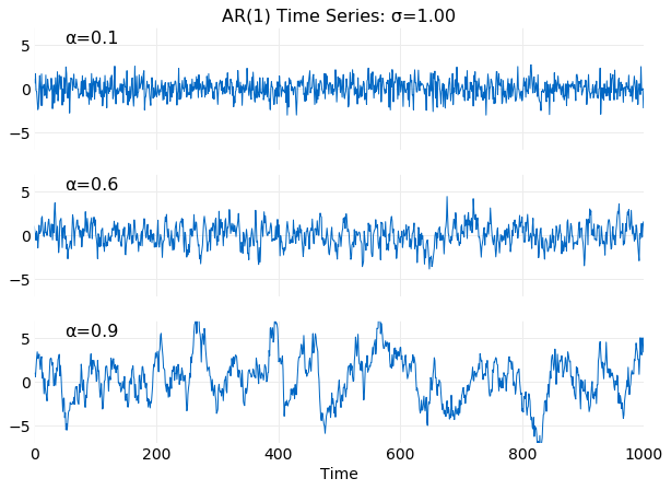
The plots below show examples of simulated time series with $\sigma=1$ and values of $\alpha$ satisfying $\alpha\ <\ 1$. It is seen that for smaller $\alpha$ values the series more frequently change direction and have smaller variance. This is expected from equation $(17)$.

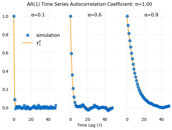
The next series of plots compare the autocorrelation coefficient from equation $(18)$, obtained in the equilibrium limit, with an autocorrelation coefficient calculation using the previously discussed autocorrelate(x) function on the generated sample data. Recall that autocorrelate(x) performs a calculation using the Cross Correlation Theorem. Equation $(18)$ does a good job of capturing the time scale for the series to become uncorrelated.

Conclusions

The Discrete Cross Correlation Theorem provides a more efficient method of calculating time series correlations than directly evaluating the sums. For a time series of length N it decreases the cost of the calculation from $O(N^2)$ to $O(NlogN)$ by use of the Fast Fourier Transform. An interpretation of the cross correlation as the time lagged covariance of two random variables was presented and followed by a discussion of the properties of Discrete Fourier Transforms needed to prove the Cross Correlation Theorem. After building sufficient tools the theorem was derived by application of the Discrete Fourier Transform to equation $(1)$, which defines cross correlation. An example manual calculation of a Discrete Fourier Transform was performed and compared with a calculation using the FFT library form numpy. Next, manual calculations of cross correlation using a tabular method to represent the summations were presented and followed by a calculation using the Discrete Cross Correlation Theorem which illustrated the problem of aliasing. The next example calculation eliminated aliasing and recovered a result equal to the direct calculation of the summations. A dealiased implementation using numpy FFT libraries was then presented. Finally, the Discrete Cross Correlation Theorem for the special case of the autocorrelation was discussed and a numpy FFT implementation was provided and followed by an example calculation using the AR(1) random process. In conclusion the autocorrelation coefficient in the equilibrium limit for AR(1) was evaluated and shown to be finite only for values of the AR(1) parameter that satisfy $\mid\alpha\mid\ < \ 1$. This result is compared to direct simulations and shown to provide a good estimate of the decorrelation time of the process.