Metropolis Hastings Sampling

Metropolis Hastings Sampling is a method for obtaining samples for a known target probability distribution using samples from some other proposal distribution. It is similar to Rejection Sampling in providing a criteria for acceptance of a proposal sample as a target sample but instead of discarding the samples that do not meet the acceptance criteria the sample from the previous time step is replicated. Another difference is that Metropolis Hastings samples are modeled as a Markov Chain where the target distribution is the Markov Chain Equilibrium Distribution. As a consequence the previous sample is used as part of the acceptance criteria when generating the next sample. It will be seen this has the advantage of permitting adjustment of some proposal distribution parameters as each sample is generated, which in effect eliminates parameter inputs.
This is is an improvement over Rejection Sampling, where it was previously shown that slight variations in proposal distribution parameters can significantly impact performance. A downside of the Markov Chain representation is that autocorrelation can develop in the samples which is not the case in Rejection Sampling.

Algorithm

The Metropolis Sampling Algorithm was developed by physicist studying simulations of equation of state at the dawn of the computer age. It is the first a a class of sampling algorithms referred to a Monte Carlo Markov Chain. A couple of decades later the algorithm was generalized and given a firmer theoretical foundation becoming the Metropolis Hastings Sampling Algorithm. After a few more decades this work became widely used in simulating Bayesian Posterior Distributions in Probabilistic Programming DSLs such as pymc. This section provides an overview of the algorithm to motivate details of the theory and examples discussed in following sections.

Let $f(y)$ denote the target distribution. The algorithm constructs a Markov Chain with equilibrium distribution, $\pi_{E}(y)$, such that,

$f(y) = \pi_{E}(y).$

The equilibrium stochastic kernel, $p(x,y)$, for the Markov Chain must satisfy,

$\pi_{E}(y) = \int_{-\infty}^{\infty} p(x, y) \pi_{E}(x) dx\ \ \ \ \ (1).$

To generate samples for $p(x, y)$ samples from a proposal Markov Chain with stochastic kernel $q(x, y)$ are produced. Let $x$ denote the state of the $p(x, y)$ Markov Chain at the previous time step, $t-1$, and $y$ represent the yet to be determined state at time $t$. Consider a proposal sample, $y^{\ast}$, generated by $q(x, y)$. Define an acceptance function, $\alpha(x, y^{\ast})$, that satisfies,

$0\ \leq\ \alpha(x, y^{\ast})\ \leq 1\ \ \ \ \ (2),$

and an acceptance random variable, $U$, with distribution $\textbf{Uniform}(0,\ 1)$ independent of $y^{\ast}$. Now, if the following inequality is satisfied,

$U\ \leq\ \alpha(x, y^{\ast}),$

accept the proposed sample, $y=y^{\ast}$, as a sample of $p(x, y)$. If the inequality is not satisfied then reject the sample by replicating the state from the previous time step, $y=x$.

It will be shown that,

$\alpha(x, y) = \text{min}\left\{\frac{f(y)q(y,x)}{f(x)q(x,y)}, 1\right\}\ \ \ \ \ (3).$

The algorithm can be summarized by the following steps that are repeated for each sample.

1. Generate samples of $y^{\ast}$ conditioned on $x$ and independently generate samples of $U$.
2. If $U\ \leq\ \alpha(x, y^{\ast})$ then $y = y^{\ast}$.
3. If $U\ >\ \alpha(x, y^{\ast})$ then $y = x$.

Theory

Metropolis Hastings Sampling is simple to implement but the theory that provides validation of the algorithm is more complicated than required for both Rejection Sampling and Inverse CDF Sampling. Here the proof that the algorithm produces the desired result is accomplished in four steps. The first will show that distributions and stochastic kernels that satisfy Time Reversal Symmetry, also referred to as Detailed Balance, are equilibrium solutions that satisfy equation $(1).$ Next, the stochastic kernel resulting from the algorithm is derived and followed by a proof that a distribution that satisfies Time Reversal Symmetry with the resulting stochastic kernel is a solution to equation $(1).$ Finally, the expression for $\alpha(x,y)$ from equation $(3)$ will be derived.

Time Reversal Symmetry

Consider a stochastic kernel $p(x,y)$ and distribution $\pi(y)$ where $x$ is the state of the Markov Chain generated by the kernel at $t-1$ and $y$ the state at time $t$. If the chain has $N$ steps the expected number of transitions from $x$ to $y$ will satisfy,

$N_{y}=N \pi(y) p(x, y).$

It follows that the rate of transition from $x$ to $y$ is given by $\pi(y) p(x,y)$. The transition rate for the Markov Chain obtained by reversing time, that is the chain transitions from $y$ to $x,$ will be $\pi(x) p(y, x)$.

Time Reversal Symmetry implies that the transition rate for the time reversed Markov Chain is the same as the forward time chain,

$\pi(y) p(x, y) = \pi(x) p(y,x)\ \ \ \ \ (3).$

If Time Reversal Symmetry is assumed it follows that,

$\begin{aligned} \int_{-\infty}^{\infty} p(x, y) \pi(x) dx &= \int_{-\infty}^{\infty} p(y, x) \pi(y) dx \\ &= \pi(y) \int_{-\infty}^{\infty} p(y, x) dx \\ &= \pi (y), \end{aligned}$

where the last step is a result of the definition of a stochastic kernel, $\int_{-\infty}^{\infty} p(y, x) dx = 1$. Thus any distribution and kernel satisfying equation $(3)$ is an equilibrium solution since it will also satisfy equation $(1)$

Stochastic Kernel

In a previous post it was shown that a stochastic kernel can be interpreted as probability density conditioned of the state at the previous time step,

$p(x,y) = f(y\mid x).$

It follows that the Cumulative Probability Distribution (CDF) of obtaining a sample $y$ for a given $x$ is given by,

$\begin{aligned} P\left[ Y\ \leq\ y\ \mid\ X=x \right] &= \int_{-\infty}^{y} f(w\mid x) dw \\ &= \int_{-\infty}^{y} p(x,w) dw. \end{aligned}$

Let $U$ represent the $\textbf{Uniform}(0, 1)$ acceptance random variable. A proposal sample, $y^{\ast}$ conditioned on $x$, is generated by $q(x,y)$ independent of $U$ and accepted if,

$U\ \leq\ \alpha(x, y^{\ast}),$

then $y=y^{\ast}$. The proposal is rejected if,

$U\ >\ \alpha(x, y^{\ast}),$

then $y=x$. Now, using the Law of Total Probability to condition on $U$ the stochastic kernel CDF becomes,

$\begin{aligned} P\left[ Y\ \leq\ y\ \mid\ X=x \right]\ &=\ P\left[Y\ \leq\ y\ \mid\ U\ \leq\ \alpha(x, y^{\ast}),\ X=x \right]\ P\left[U\ \leq\ \alpha(x, y^{\ast})\ \mid\ X=x \right] \\ &\ + P\left[Y\ \leq\ y\ \mid\ U\ >\ \alpha(x, y^{\ast}),\ X=x \right]\ P\left[U\ >\ \alpha(x, y^{\ast})\ \mid\ X=x \right]. \end{aligned}\ \ \ \ \ (4).$

The first term is the probability that the proposed sample is accepted and the second term the probability that it is rejected. Consider the first term where $U\ \leq\ \alpha(x, y^{\ast})$ and $y=y^{\ast}$,

$P\left[Y\ \leq\ y,\ U\ \leq\ \alpha(x, y^{\ast})\ \mid\ X=x \right]\ =\ P\left[Y\ \leq\ y\ \mid\ U\ \leq\ \alpha(x, y^{\ast}),\ X=x \right]\ P\left[U\ \leq\ \alpha(x, y^{\ast})\ \mid\ X=x \right]\ \ \ \ \ (5),$

which follows from the definition of Conditional Probability.

The algorithm assumes that $U$ is independent of $y^{\ast}$ conditioned on $x$. It follows that the joint density is given by,

$\begin{aligned} h(y^{\ast}, u\mid x) &= g(u)f(y^{\ast}\mid x) \\ &= q(x, y^{\ast}), \end{aligned}$

where the last step follows by noting that since $U\ \sim\ \textbf{Uniform}(0,1),$ the density of $U$ is given by $g(u)=1$ and the density of $y^{\ast}$ conditioned on $x$ is given by the proposal stochastic kernel, $f(y^{\ast}\mid x)=q(x, y^{\ast}).$ Using this result to continue gives the acceptance probability term for the stochastic kernel CDF from equation $(5)$,

$\begin{aligned} P\left[Y\ \leq\ y,\ U\ \leq\ \alpha(x, y^{\ast})\ \mid\ X=x \right] &= \int_{-\infty}^{y}\int_{0}^{\alpha(x, y^{\ast})} h(y^{\ast}, u\mid x) du dy^{\ast} \\ &= \int_{-\infty}^{y}\int_{0}^{\alpha(x, y^{\ast})} q(x, y^{\ast}) du dy^{\ast} \\ & = \int_{-\infty}^{y} \alpha(x, y^{\ast}) q(x, y^{\ast}) dy^{\ast} \end{aligned}\ \ \ \ \ (6).$

Next, consider the second term in equation $(4)$, which represents the case where $y^{\ast}$ is rejected as a sample of $y$. Since $y^{\ast}$ is rejected $y=x$. It follows that any value of $y^{\ast}$ is possible so the integral over $y^{\ast}$ needs to be over its entire range. Using the previous result for the joint density $h(y^{\ast}, u\mid x)$. gives

$\begin{aligned} P\left[Y\ = x,\ U\ >\ \alpha(x, y^{\ast})\ \mid\ X=x \right] &= \int_{-\infty}^{\infty}\int_{\alpha(x, y^{\ast})}^{1} h(y^{\ast}, u\mid x) du dy^{\ast} \\ &= \int_{-\infty}^{\infty}\int_{\alpha(x, y^{\ast})}^{1} q(x, y^{\ast}) du dy^{\ast} \\ &= \int_{-\infty}^{\infty}\left[ 1-\alpha(x, y^{\ast})\right] q(x, y^{\ast}) dy^{\ast} \\ &= \int_{-\infty}^{\infty}\ q(x, y^{\ast}) dy^{\ast} - \int_{-\infty}^{\infty}\alpha(x, y^{\ast}) q(x, y^{\ast}) dy^{\ast} \\ &= 1 - \int_{-\infty}^{\infty}\alpha(x, y^{\ast}) q(x, y^{\ast}) dy^{\ast} \end{aligned}\ \ \ \ \ (7)$

since $\int_{-\infty}^{\infty}\ q(x, y^{\ast}) dy^{\ast}=1$. Simplify things by defining the rejection probability density by,

$f_{R}(x) = 1 - \int_{-\infty}^{\infty}\alpha(x, y) q(x, y) dy\ \ \ \ \ (8).$

Equation $(7)$ needs to be written as an integral over $y$ to continue with the evaluation of equation $(4)$. This is accomplished by use of the Dirac Delta Function which is defined by,

$\int_{-\infty}^{\infty} f(y^{\ast})\delta(y^{\ast}-x) dy^{\ast} = f(x).$

If use is made of equation $(8)$ and the Dirac Delta Function it follows that equation $(7)$ becomes,

$P\left[Y\ \leq\ y,\ U\ >\ \alpha(x, y^{\ast})\ \mid\ X=x \right] = \int_{-\infty}^{y} f_{R}(y^{\ast})\delta(y^{\ast}-x) dy^{\ast}\ \ \ \ \ (9).$

The upper range of the limit was changed to conform to the limits of the CDF. This is acceptable since if $y\ <\ x$ the probability of rejection is 0. The Metropolis Hastings stochastic kernel can now by constructed by assembling the results obtained in equations $(6)$ and $(9)$ and revisiting equation $(5)$,

$\begin{aligned} \int_{-\infty}^{y} p(x,w) dw & = P\left[ Y\ \leq\ y\ \mid\ X=x \right] \\ &= P\left[Y\ \leq\ y,\ U\ \leq\ \alpha(x, y^{\ast})\ \mid\ X=x \right] + P\left[Y\ \leq\ y,\ U\ >\ \alpha(x, y^{\ast})\ \mid\ X=x \right] \\ &= \int_{-\infty}^{y} \alpha(x, y^{\ast}) q(x, y^{\ast}) dy^{\ast} + \int_{-\infty}^{y} f_{R}(y^{\ast})\delta(y^{\ast}-x) dy^{\ast} \\ &= \int_{-\infty}^{y} \left[ \alpha(x, y^{\ast}) q(x, y^{\ast}) + f_{R}(y^{\ast})\delta(y^{\ast}-x)\right] dy^{\ast} \end{aligned}$

Finally, the desired result is obtained by collecting the terms under a single integration variable,

$\begin{gathered} p(x,y) = \alpha(x, y) q(x, y) + f_{R}(y)\delta(y-x) \\ f_{R}(x) = 1 - \int_{-\infty}^{\infty}\alpha(x, y) q(x, y) dy \end{gathered}\ \ \ \ \ (10)$

Verify that the kernel satisfies the stochastic property,

$\begin{aligned} \int_{-\infty}^{\infty} p(x,y) dy &= \int_{-\infty}^{\infty}\left[ \alpha(x, y) q(x, y) + f_{R}(y)\delta(y-x)\right] dy \\ &= \int_{-\infty}^{\infty}\alpha(x, y) q(x, y) dy - f_{R}(x) \\ &= \int_{-\infty}^{\infty}\alpha(x, y) q(x, y) dy + 1 - \int_{-\infty}^{\infty}\alpha(x, y) q(x, y) dy \\ &= 1 \end{aligned}$

which is the desired result.

Equilibrium

It can now be shown that the Metropolis Hastings stochastic kernel from equation $(10)$ is an equilibrium solution by evaluating the integral from equation $(1)$ that defines equilibrium. Additionally, Time Reversal Symmetry must also be assumed,

$\pi(x)\alpha(x,y)q(x,y) = \pi(y)\alpha(y,x)q(y,x)\ \ \ \ \ (11),$

where $\alpha(x,y)$ is the acceptance function from equation $(1)$, $q(x,y)$ is the stochastic kernel for the proposal Markov Chain, $\pi(y)$ is the distribution, $y$ is the state of the target Markov Chain at time step $t$ and $x$ the state at time $t-1$.

Now, starting with equation $(1)$,

$\begin{aligned} \int_{-\infty}^{\infty} p(x, y) \pi(x) dx &= \int_{-\infty}^{\infty}\left[ \alpha(x, y) q(x, y) + f_{R}(y)\delta(y-x)\right] \pi(x) dx \\ &= \int_{-\infty}^{\infty}\alpha(x, y) q(x, y) \pi(x) dx + f_{R}(y)\pi(y) \\ &= \int_{-\infty}^{\infty}\alpha(x, y) q(x, y) \pi(x) dx + \left[1 - \int_{-\infty}^{\infty}\alpha(y, w) q(y, w) dw \right]\pi(y) \\ &= \pi(y)+\int_{-\infty}^{\infty}\alpha(x, y) q(x, y) \pi(x) dx - \int_{-\infty}^{\infty}\pi(y)\alpha(y, w) q(y, w) dw \\ &= \pi(y)+\int_{-\infty}^{\infty}\alpha(x, y) q(x, y) \pi(x) dx - \int_{-\infty}^{\infty}\pi(w)\alpha(w, y) q(w, y) dw \\ &= \pi(y), \end{aligned}$

where the last steps follow from substituting equation $(11)$ into the last term leading to the desired result.

Derivation of $\alpha(x,y)$

It has been shown that the Metropolis Hastings algorithm generates a Markov Chain with an equilibrium distribution equal to the target distribution. This has been accomplished by only requiring that the acceptance function, $\alpha(x,y)$, satisfy Time Reversal Symmetry as specified by equation $(11)$ without giving and explicit form. Here an expression for $\alpha(x,y)$ is derived with the aim of driving arbitrary proposal Markov Chains toward states satisfying Time Reversal Symmetry.

For an arbitrary proposal stochastic kernel, $q(x,y)$, Time Reversal Symmetry will not be satisfied, so either $\pi(x)q(x,y)\ >\ \pi(y)q(y,x)$ or $\pi(x)q(x,y)\ <\ \pi(y)q(y,x)$ will be true. Assume the first condition is valid. If this is the case transitions from $x$ to $y$ occur more frequently than transitions from $y$ to $x$. To correct for the imbalance the number of transitions from $x$ to $y$ needs to be decreased and the number of transition from $y$ to $x$ increased. This can be accomplished by setting $\alpha(y,x)=1$ in equation $(11)$ to obtain,

$\pi(x)\alpha(x,y)q(x,y) = \pi(y)q(y,x).$

Solving this equation for $\alpha(x,y)$ gives,

$\alpha(x,y) = \frac{\pi(y)q(y,x)}{\pi(x)q(x,y)}.$

Similarly if the second condition, $\pi(x)q(x,y)\ <\ \pi(y)q(y,x)$, is satisfied by the proposal stochastic kernel the number of transitions from $x$ to $y$ needs to be increased and the transitions from $y$ to $x$ decreased. Setting $\alpha(x,y)=1$ in equation $(11)$ produces the desired result,

$\pi(x)q(x,y) = \pi(y)\alpha(y,x)q(y,x).$

Solving for $\alpha(y,x)$ gives,

$\alpha(y,x) = \frac{\pi(x)q(x,y)}{\pi(y)q(y,x)},$

which is the time reversed version of the first result. Equation $(3)$ follows when the constraint, $0\ \leq\ \alpha(x, y^{\ast})\ \leq 1,$ is considered,

$\alpha(x, y) = \text{min}\left\{\frac{f(y)q(y,x)}{f(x)q(x,y)}, 1\right\}.$

Example

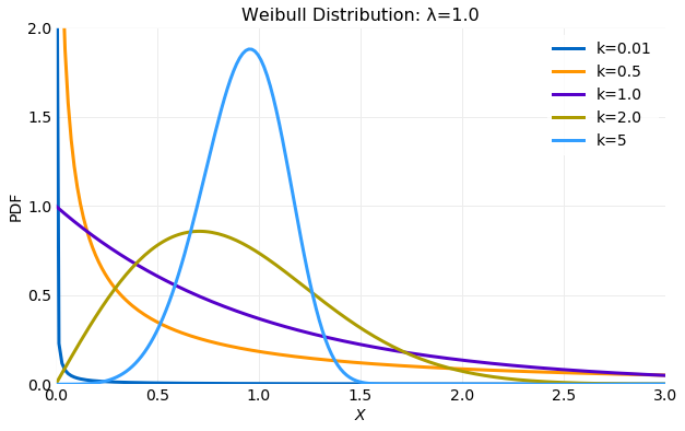
Here an example implementation of the Metropolis Hastings Sampling algorithm using a $\textbf{Weibull}$ target distribution and $\textbf{Normal}$ proposal distribution is discussed. The $\textbf{Weibull}$ distribution PDF is defined by,

$f_X(x; k, \lambda) = \begin{cases} \frac{k}{\lambda}\left(\frac{x}{\lambda} \right)^{k-1} e^{-\left(x/\lambda\right)^k} & x\ \geq\ 0 \\ 0 & x < 0 \end{cases} \ \ \ \ \ (12),$

where $k\ >\ 0$ is the shape parameter and $\lambda\ >\ 0$ the scale parameter. The first and second moments are,

$\begin{aligned} \mu & = \lambda\Gamma\left(1+\frac{1}{k}\right) \\ \sigma^2 & = \lambda^2\left[\Gamma\left(1+\frac{2}{k}\right)-\left(\Gamma\left(1+\frac{1}{k}\right)\right)^2\right] \end{aligned} \ \ \ \ \ (13),$

where $\Gamma(x)$ is the Gamma function. The following plot illustrates the variation in the $\textbf{Weibull}$ distribution for a fixed value of the scale parameter of $\lambda=1$ as the shape parameter, $k$, is varied. The following sections will assume that $\lambda=1$ and $k=5$.

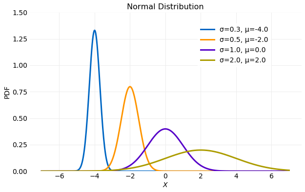
The Normal distribution is defined by the PDF,

$f_X(x; \mu, \sigma^2) =\frac{1}{\sqrt{2\pi\sigma^2}}e^{(x-\mu)^2/2\sigma^2}\ \ \ \ \ (14),$

where $\mu$ is the location parameter and first moment and $\sigma^2$ is the scale parameter and second moment. The following plot illustrates variation in the PDF as the scale and location parameter are varied.

Proposal Distribution Stochastic Kernel

The Metropolis Hastings Sampling algorithm requires a stochastic kernel based on the proposal distribution. A $\textbf{Normal}$ stochastic kernel can be derived from the difference equation,

$X_{t} = X_{t-1} + \varepsilon_{t},$

where $t=0,\ 1,\ 2,\ldots$ and the $\varepsilon_{t}$ are identically distributed independent $\textbf{Normal}$ random variables with zero mean and variance, $\sigma^2$. Let $y=X_{t}$ and $x=X_{t-1}$ then the equation above becomes,

$y-x=\varepsilon_{t}.$

Substitution into equation $(14)$ gives the stochastic kernel,

$q(x,y) = \frac{1}{\sqrt{2\pi\sigma^2}} e^{-(y-x)^2/2\sigma^2}\ \ \ \ \ (15),$

The form of $q(x,y)$ is a $\textbf{Normal}$ distribution with mean $\mu=x$. This has eliminated $\mu$ as a free parameter. The only arbitrary parameter is the standard deviation, $\sigma$. In the implementation $\sigma$ will be referred to as the stepsize. The plot below shows how $q(x,y)$ varies with each step in a simulation. The first five steps are shown for an initial condition $X_{0}=0$ and stepsize=1.0.

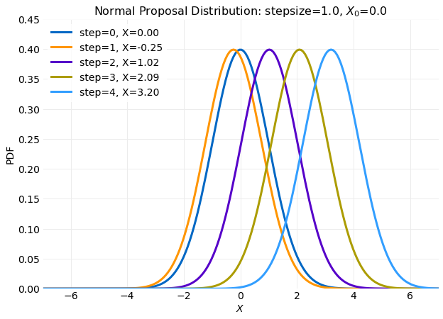
In the plot it is seen that the distribution is recentered at each step about the the previous value. This behavior is a consequence of the assuming a $\textbf{Normal}$ proposal distribution. Using another form for a proposal distribution could use a different parameterization.

A Rejection Sampling implementation using the same proposal and target distributions has both $\mu$ and $\sigma$ as arbitrary parameters. Modeling the sampling process as a Markov Chain has eliminated one parameter.

Implementation

Metropolis Hastings Sampling is simple to implement. This section will describe an implementation in Python using libraries available in numpy. Below a sampler for $q(x,y)$ using the numpy normal random number generator is shown.

import numpy

def qsample(x, stepsize):
    return numpy.random.normal(x, stepsize)

qsample(x, stepsize) takes two arguments as input. The first is x, the previous state, and the second the stepsize. x is used as the loc parameter and stepsize the scale parameter in the call to the numpy normal random number generator.

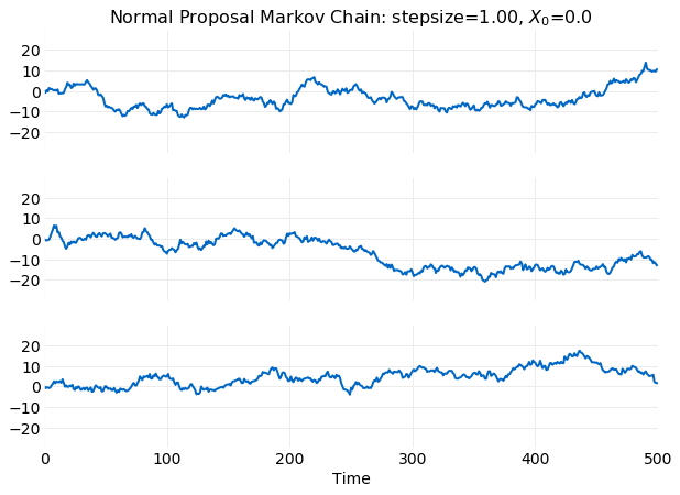
Simulations of time series using qsample(x, stepsize) can be performed using the code below.

stepsize = 1.0
x0 = 0.0
nsamples = 500
x = numpy.zero(nsamples)

x[0] = x0
for j in range(1, nsamples):
    x[j] = qsample(x[j-1], stepsize)

The following plot shows time series generated by three separate runs of the code listed above.

The Python implementation of the algorithm summarized in the Algorithm section is shown below,

def metropolis_hastings(f, q, qsample, stepsize, nsample, x0):
    x = x0
    samples = numpy.zeros(nsample)
    for i in range(nsample):
        u = numpy.random.rand()
        y_star = qsample(x, stepsize)
        fy_star = f(y_star)
        fx = p(x)
        α = (fy_star*q(y_star, x, stepsize)) / (fx*q(x, y_star, stepsize))
        if u < α:
            x = y_star
        samples[i] = x
    return samples

metropolis_hastings(f, q, qsample, stepsize, nsample, x0) takes five arguments as input that are described in the table below.

Argument	Description
f	The target distribution which is assumed to support an interface taking a the previous state, x, as a floating point argument. In this example equation $(12)$ is used.
q	The proposal stochastic kernel which is assumed to support an interface taking the previous state, x, and the stepsize both as floating point arguments. In this example equation $(15)$ is used.
qsample	A random number generator based on the proposal stochastic kernel, $q(x,y).$ It is assumed to support an interface taking the previous state, x, and the stepsize both as floating point arguments. The implementation used in this example is the function qsample(x, stepsize) previously discussed.
stepsize	The scale parameter used by the proposal distribution.
nsample	The number of samples desired.
x0	The initial target sample value.

The execution of metropolis_hastings(f, q, qsample, stepsize, nsample, x0) begins by allocation of storage for the result and initialization of the Markov Chain. A loop is then executed nsample times where each iteration generates the next sample. Within the loop the acceptance random variable with distribution $\textbf{Uniform}(0,\ 1)$ is generated using the numpy random number generator. Next, a proposal sample is generated using qsample(x, stepsize) followed by evaluation of the acceptance function $\alpha(x,y)$. Finally, the acceptance criteria is evaluated leading the sample being rejected or accepted.

Simulations

Here the results of simulations performed using,

 metropolis_hastings(f, q, qsample, stepsize, nsample, x0),

from the previous section are discussed. The simulations assume the $\textbf{Weibull}$ target distribution from equation $(12)$ with $\lambda=1$ and $k=5$ and the $\textbf{Normal}$ stochastic kernel from equation $(14)$. First, simulations that scan 4 orders of magnitude of stepsize with x0 fixed are compared with the goal of determining the value leading to the best performance. Next, simulations are performed with stepsize fixed that scan values of x0 to determine the impact of initial condition on performance. Finally, a method for removing autocorrelation from generated samples using Thinning is discussed.

The criteria for evaluating simulations include the time for convergence of the first and seconds moments computed from samples to the target distribution moments, the fit of the sampled distribution to the target PDF, the percentage of accepted proposal samples and the timescale for the decay of time series autocorrelation. It will be shown that stepsize is the only relevant parameter. The choice for x0 will be seen to have an impact that vanishes given sufficient time. Thus, the model has a single parameter of significance.

Performance

The plot below shows the percentage of proposal samples accepted as a function of stepsize for simulations with stepsize ranging from $10^{-3}$ to $10^{1}$. For all simulations x0=1.0. The simulation believed to be the best performing accepted $82\%$ of the proposed samples and had a stepsize of $0.12$. The two other simulations discussed in this section as representative of small and large values of stepsize had acceptance percentages of $99\%$ and $19\%$ for stepsize values of $0.01$ and $1.33$ respectively. Each of this simulations is indicated in the plot below.

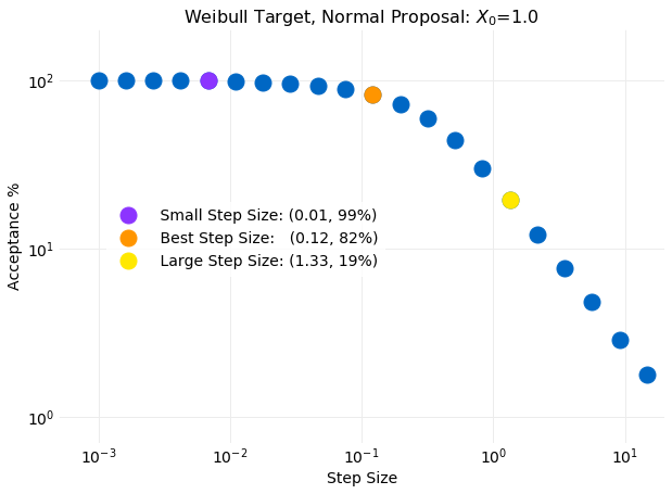
On examination of the plot it is seen that for stepsize smaller than $0.12$, the simulations to the left of the orange symbol, the accepted percentage of proposal samples very quickly approach $100\%$ while for stepsize larger than $0.12$, the simulations to the right of the orange symbol, the accepted percentage approaches $0\%$ as a power law.

To get a sense of why this happens the stepsize is compared to the standard deviation of the target distribution computed from equation $(13)$, using the assumed values for $\lambda$ and $k$, gives $0.21$. This value is the same order of magnitude of the best performing stepsize determined from simulations. Comparing the stepsize to the target standard deviation in the large and small limits provides an interpretation of the results. For small stepsize relative to the target standard deviation the proposal variance is much smaller then the target variance. Because of this the steps taken by the proposal Markov Chain are small leading to a exploration of the target distribution that never goes far from the initial value. The samples produced will have the proposal distribution since nearly all proposals are accepted. 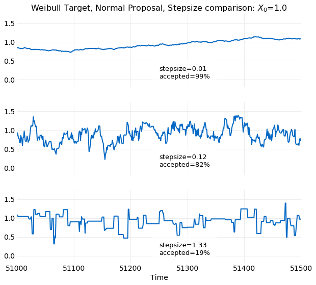This is seen in the first of the following plots where time series examples for different stepsize values for the last $500$ steps for a $51000$ sample simulation are shown. The small variance seen in the first plot is a consequence of the small stepsize leading to very small deviations from the initial value x0=1. In the opposite limit where the stepsize becomes large relative to the target standard deviation the steps taken by the proposal Markov Chain are so large that they are frequently rejected since low probability target events are oversampled. This effect is seen in last time series plot shown below. There long runs where the series has a constant value are clearly visible. The best value of stepsize relative to the target standard deviation occurs when they are about the same size. The middle plot below has the optimal stepsize of $0.12$ and accepted $82\%$ of the proposed samples. It clearly has a more authentic look than the other two simulations which are at extreme values of the percentage accepted.

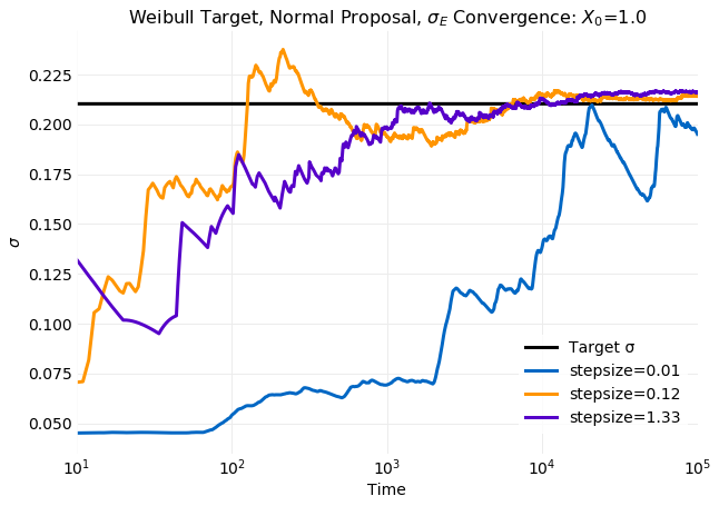
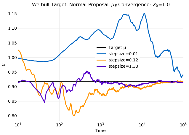
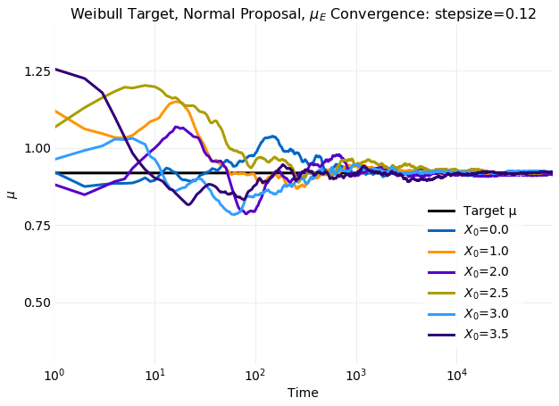
A measure of simulation performance is the rate of convergence of distribution moments computed from samples to the target distribution momements. The next two plots show convergence of the cumulative sample mean, $\mu$, and standard deviation, $\sigma$, to the target distribution values computed from equation $(13)$ for three values of stepsize that compare simulations at both the small and large extremes with the optimal stepsize of $0.12$. For both $\mu$ and $\sigma$ the small stepsize example is clearly the worst performing. After $10^5$ time steps there is no indication of convergence. There is no significant difference between the other two simulations. Both are showing convergence after $O(10^4)$ samples.

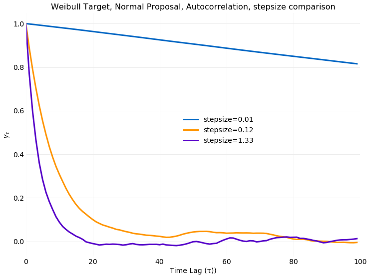
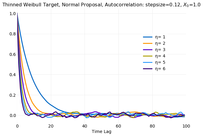
A consequence of using a Markov Chain to generate samples is that autocorrelation is built into the model. This is considered an undesirable artifact since in general independent and identically distributed samples are desired. It follows that there is a preference for rapid decorrelation of samples. The following plot shows the autocorrelation coefficient for the three values of stepsize previously discussed. The autocorrelation coefficient of a time series, $f$, provides a measure of similarity or dependence of the series past and future and is defined by,

$\gamma_{\tau} = \frac{1}{\sigma_{f}^2}\sum_{n=0}^{t} \left(f_{n} - \mu_f \right) \left(f_{n+\tau} - \mu_f\right),$

where $\mu_{f}$ and $\sigma_{f}$ are the time series mean and standard deviation respectively. Calculation of autocorrelation was discussed in a previous post. The small stepsize simulation has a very slowly decaying autocorrelation. For time lags of up to 100 steps it has decayed by only a few precent. This behavior is expected since for small stepsize the resulting samples are from the proposal Markov Chain, with stochastic kernel shown in equation $(15)$, which has an autocorrelation coefficient independent of $\tau$ given by $\gamma_{\tau}=1$. The other simulations have a similar decorrelation rate of $O(10)$ time steps, though for the larger stepsize the decorrelation rate is slightly faster.

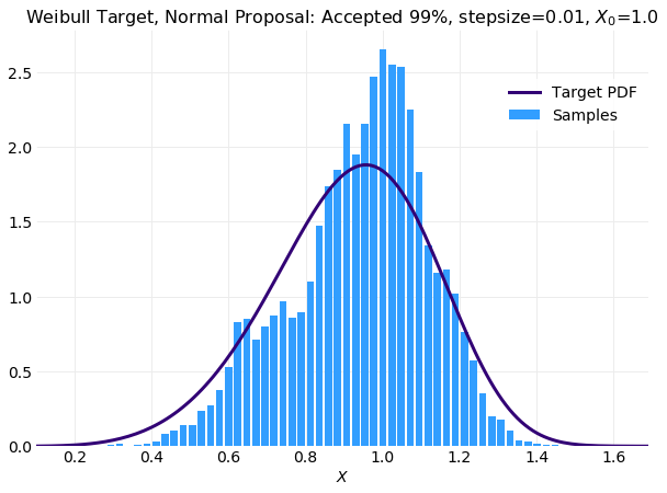
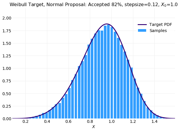
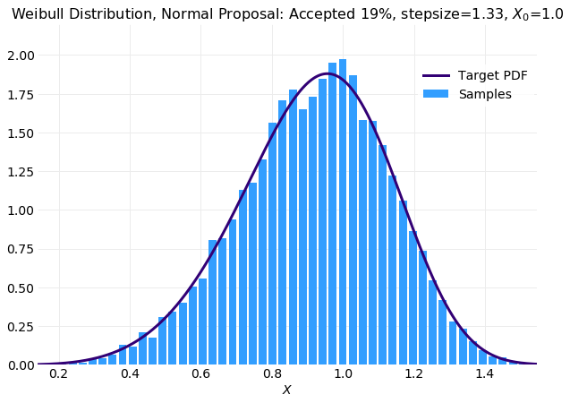
The following three plots compare histograms computed from simulations of $10^5$ samples with the target $\textbf{Weibull}$ distribution from equation $(12)$ for the same stepsize values used in the previous comparisons. The first plot shows the small stepsize simulation with a very high acceptance rate. For this case the simulated histogram is not close to reproducing the target distribution. The last plot is the large stepsize simulation with a very large rejection rate. When compared with optimal stepsize of $0.12$ simulation shown in the middle plot the larger stepsize simulation is not as smooth but is acceptable. The degraded performance of larger stepsize simulation will be a consequence of rejection of many more proposal samples leading to long stretches of repeated values. For the optimal stepsize simulation almost $10$ times more samples are available in the histogram calculation.

In summary a collection of simulations using the Metropolis Hastings Sampling algorithm to sample a target $\textbf{Weibull}$ distribution using a $\textbf{Normal}$ proposal distribution have been performed that scan the stepsize parameter for a fixed initial value of x0=1.0 in an effort to determine the best performing stepsize. Best performing was determined by considering the total percentage of accepted samples, the quality of the generated time series, the convergence of first and second moments to the known target values, the decorrelation timescale and fit of sample histograms to the target distribution. The best performing stepsize was found to have a value of $0.12$ which is near the standard deviation of the target distribution. For values of stepsize smaller than the best performing stepsize the performance was inferior on all counts. The number of accepted proposals was high, the time series look like the proposal distribution, convergence of moments is slow, samples remain correlated over long time scales and the distributions computed from samples do not converge to the target distribution. When the same comparison is made to simulations with a larger stepsize the results were less conclusive. Larger values of stepsize accept fewer proposal samples. This causes degradation of the time series since there are many long runs of repeated values. In comparisons of convergence of distribution moments and autocorrelation there was no significant differences but calculation of the distribution using histograms on sample data were not as acceptable since an order of magnitude less data was used in the calculation because of the high rejection percentage.

Burn In

In the previous section simulations were compared that scanned stepsize with x0 fixed. Here simulations with stepsize fixed that scan x0 are discussed. The further x0 is from the target distribution mean the further displaced the initial state is from equilibrium so the expectation is that a longer time is required to reach equilibrium. If some knowledge of the target mean is available it should be used to minimize this relaxation period. The time required to reach equilibrium is referred to as burn in. Typically the burn in period of the simulation is considered and artifact and discarded with the aim of improving the final result. The expectation then is that the simulation is generating natural fluctuations about equilibrium.

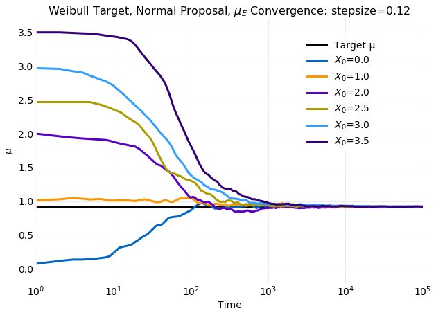
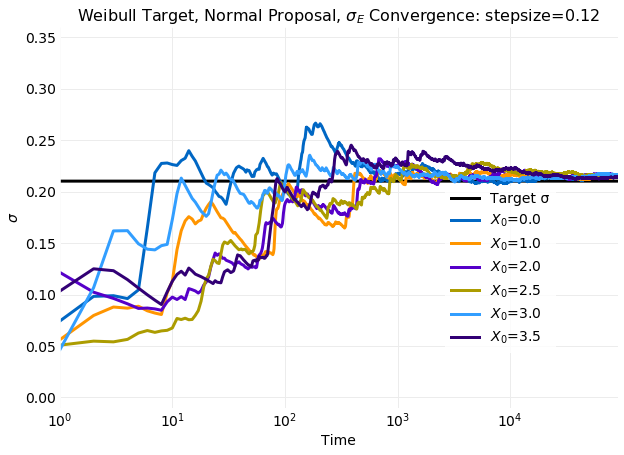
The two plots above compare cumulative first and second moment calculations on simulated samples with the target $\textbf{Weibull}$ distribution values calculated from equation $(13)$ using $\lambda = 1$ and $k=5$. The obtained mean and standard deviation are $0.92$ and $0.21$ respectively. In the plots time to reach equilibrium in seen to increase with increasing displacement of x0 from $0.92$. For the simulation at the most extreme value of x0 the time to reach equilibrium is a factor of $10$ longer than the simulation that reached equilibrium first. 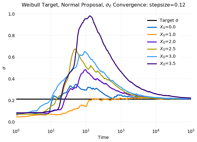For standard deviation the effect is even larger increasing the relaxation time by nearly a factor of $10^2$ when compared to the fastest relaxation time seen. There is also a very large spike in the standard deviation that increases with displacement of x0 from the target mean.

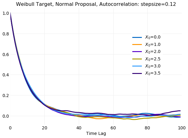
The following plot of the autocorrelation coefficient shows that time for sampled time series to decorrelate is not impacted by the initial value of x0.

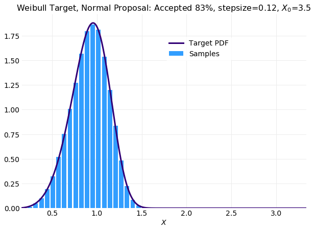
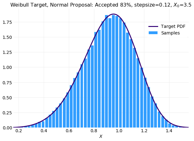
The next plot shows a comparison of the histogram computed from the worst performing simulation with x0=3.5 with the target distribution. The over representation of large low probability samples induced by the large displacement of the initial condition is apparent in the long right tail.

In the next series of plots a burn in period of $10^4$ time steps is assumed and the data is excluded from calculations. This corresponds to removing $20\%$ of the samples. The magnitude of the adjustment to equilibrium is significantly reduced. Within $10^3$ time steps all simulations for both moments are near their equilibrium values with no significant difference in the convergence rate. The clear increase in the time of convergence to equilibrium with displacement of x0 from the equilibrium value seen when all samples are included has been eliminated.

The final plot compares the sample histogram with burn in removed for the simulation with x0=3.5 to the target distribution. It is much improved from the plot in which burn in was retained. In fact it is comparable with the same plot obtained for a simulation where x0=1 above.

Thinning

It is desirable that sampling algorithms not introduce correlations between samples since random number generators for a given distribution are expected to produce independent and identically distributed. Since Metropolis Hastings Sampling models generated samples as a Markov Chain, autocorrelation is expected because the proposal stochastic kernel depends on the previously generated sample. Thinning is a method for reducing autocorrelation in sequence of generated samples. It is a simple algorithm that can be understood by considering a time series $\{x_{t}\}$ samples of length $N$. Thinning discards samples that do not satisfy $t\ \mod\ {\eta}=0$, where $\eta$ is referred to as the thinning interval. Discarding all but equally spaced samples increases the time between the retained samples which can reduce autocorrelation.

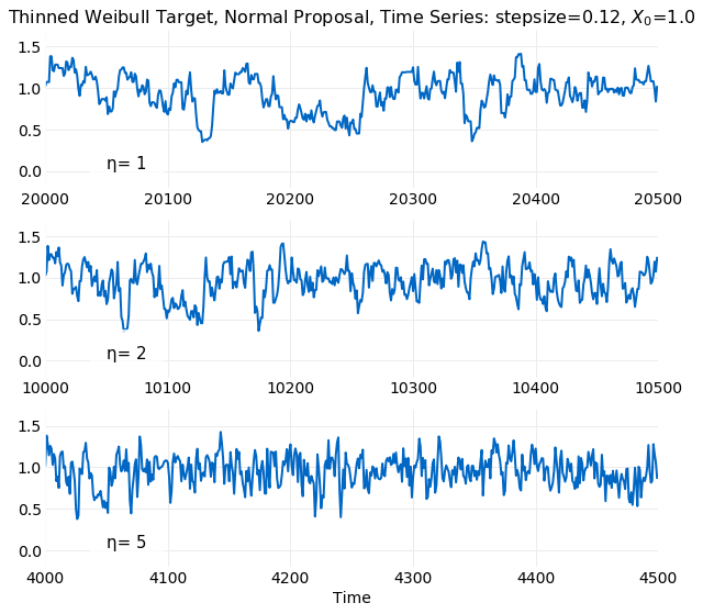
The impact of Thinning on the appearance of the time series is illustrated below. The first plot is from the original time series and the others illustrate increasing the thinning interval. The first point in each plot is the same and the plot range is adjusted so that all have $500$ samples. A tendency of series values to infrequently change from increasing to decreasing as time increases is an indication of autocorrelation. Comparison of the original series with the thinned series illustrates this. The plot with $\eta=1$ may have runs of $O(10)$ samples with a persistent increasing or decreasing trend which is consistent with decorrelation time of $O(10)$ previously demonstrated. For increasing $\eta$ the length of increasing or decreasing trends clearly decreases.

The following plot confirms this intuition. The simulation samples are generated using Metropolis Hastings with a $\textbf{Weibull}$ target distribution and $\textbf{Normal}$ proposal distribution with x0=1 and the previously determined best performing stepsize=0.12. The burn in period samples have also been discarded. A value of $\eta=1$ corresponds to not discarding any samples. It is seen that the decorrelation time scale decreases rapidly with most of the reduction occurring by $\eta=4.$

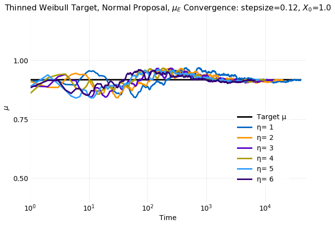
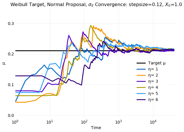
Thinning has no impact on the rate of convergence of first and second moments computed from samples to the target distribution values. This is shown in the following two plots which have convergence rates of $O(10^3)$ samples as seen in the previous section when only the burn in samples were discarded.

The following two plots compare histograms computed from samples with the target distribution for different values of the thinning interval. The first plot shows the original series and the second the result from thinned samples. The fit of the thinned plot is degraded but this will be due to the smaller number on samples. The original series consists of $4\times 10^4$ samples and the thinned series $6.6\times 10^3$. It follows that if fairly aggressive thinning is performed simulations may need to be run $O(10)$ longer to obtain a sufficient set of samples.

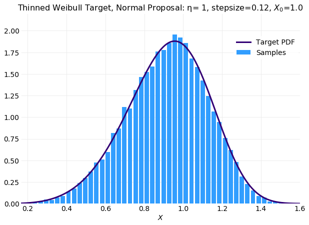
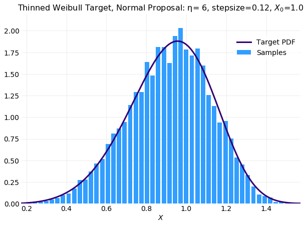
The following plot shows the results of a simulation $5\times10^5$ samples that is comparable with the result obtained without thinning.

Conclusions

The Metropolis Hastings Sampling algorithm provides a general method for generating samples for a known target distribution using an available proposal sampler. The algorithm is similar to Rejection Sampling but instead of discarding rejected proposal samples Metropolis Hastings Sampling replicates the previous sample. It also has a more complicated acceptance function that assumes the generated samples are a Markov Chain. Metropolis Hastings Sampling is simple to implement but the theory describing how it works is more sophisticated than that encountered in both Inverse CDF Sampling and Rejection Sampling.

The theoretical discussion began by deriving the stochastic kernel following from the assumptions introduced by the rejection algorithm, equation $(10)$. Next, it was shown that if Time Reversal Symmetry were assumed for the stochastic kernel and target distribution, equation $(11)$, then the target distribution is the equilibrium distribution of the Markov Chain created by the stochastic kernel. Finally, the acceptance function, equation $(3)$, was derived using Time Reversal Symmetry.

A Python implementation of a Metropolis Hastings Sampler was presented and followed by discussion of an example using a $\textbf{Weibull}$ distribution as target and a $\textbf{Normal}$ distribution as proposal. A parameterization of the proposal stochastic kernel using setpsize as the standard deviation of the proposal distribution was described. The results of a series of simulations that varied stepsize for a fixed initial state, x0, over several orders of magnitude were presented. It was shown that the best performing simulations have stepsize that is about the same as the standard deviation of the proposal distribution. This was followed by simulations that scanned x0 for the stepsize determined as best. It was shown that the best performing simulations have x0 near the mean of the target distribution but that if the first $10^4$ samples of the simulation were discarded x0 can differ significantly from the target mean with no impact. Autocorrelation of samples is a consequence of using a Markov Chain to model samples and considered an undesirable artifact since independent identically distributed samples are desired. Autocorrelation can be removed by Thinning the samples. It was shown that thinning intervals of about $\eta=5$ can produce samples with a very short decorrelation time at the expense of requiring generation of more samples.

The best performing simulations using Metropolis Hastings Sampling have an acceptance rate of about $80\%$ and converge to target values in about $O(10^3)$ time steps. This is the same performance obtained using Rejection Sampling with a $\textbf{Normal}$ proposal distribution. The advantage offered by Metropolis Hastings Sampling is that it has a single arbitrary parameter. Rejection sampling has two arbitrary parameters that can significantly impact performance for small changes. It follows that Metropolis Hastings Sampling can be considered more robust.